Computer Modelers Stimulate Real and Potential Climate, Work Toward Prediction
Combining Equations and Data Pushes Computers' Limits
December 1996 — Although weather forecasting is accepted by the public as part of daily life, oceanic forecasting is not yet so advanced. There are, however, successful examples of oceanic forecasting—one is the newly developed skill to predict El Niño/Southern Oscillation (ENSO) events, largely due to improvements in ocean modeling (see Lewis Rothstein article).
In 1982 and 1983, Eastern Australia and Indonesia experienced the century’s worst drought, which led to devastation in agricultural regions and rain forests, and even to loss of hundreds of lives. These were just some regional impacts of what is now known as the most severe ENSO event on record, an anomalous warming of sea surface temperature in the eastern Tropical Pacific Ocean that occurs once every three to seven years. The change in oceanic conditions associated with ENSO is usually accompanied by atmospheric shifts, and together these phenomena lead to droughts in some parts of the world and flooding in others. It is estimated that total worldwide damage caused by the 1982-83 ENSO was more than $10 billion./p>
Another climate variation, the North Atlantic Oscillation (NAO), a shift of atmospheric pressure fields between Iceland (65°N) and the Azores (40°N) on decadal time scales, is known to change weather conditions in Europe and North America (see NAO inset in Clara Deser’s article). ENSO and NAO are just two examples of how natural climatic fluctuations can dramatically affect the world economy and our daily lives. Earth’s climate changes ceaselessly, and it will surely continue to evolve, possibly in a more complicated manner due to increasing atmospheric concentrations of greenhouse gases. Thus there are pressing reasons to improve our understanding of severe climate variations, such as ENSO and NAO events, and even to predict them before they occur so that the public can be informed and policy makers can prepare for possible natural disasters. Because the future is unobservable, we must rely on numerical models for such forecasting.
Geologic studies of Earth’s history show that the world ocean has changed profoundly over time. Modern observations indicate that there have been noticeable changes in world ocean circulation even during recent decades. As our knowledge advances, so does our understanding of the ocean’s importance in the climate system. Driven by wind stress as well as heat and freshwater fluxes, oceanic currents redistribute heat across the globe and regulate our climate. The ocean’s enormous capacity to store heat also buffers climate changes. Since the ocean and the atmosphere exchange momentum, heat, and fresh water across their interfaces, variation in one fluid system can lead to changes in the other, often in a chain reaction that amplifies initially small deviations. Many climate phenomena, such as ENSO, result from such interactions, which can occur over a wide spectrum of time scales. So, even though the weather can be forecast for a week without considering oceanic circulation, climate on time scales longer than a month must include the ocean.
Temporal evolution and spatial variation of the ocean are constrained by physical laws and such external forcing fields as wind stresses and surface buoyancy fluxes. The essence of climate modeling is to integrate the dynamic equations for these climate components forward in time, starting with conditions that are often based on actual observations. The basic idea of computer simulation is to organize physical equations into a net of grids arranged to cover a spatial domain, such as the tropical Pacific Ocean for ENSO predictions, or the global oceans for carbon cycle assessments, and then predict the climatic state at each grid in the future based on its initial condition and its subsequent interactions with surrounding grids as the conditions in each change. Though the evolution of a climate event is unrepeatable and beyond our control, computer simulations can be repeated many times by varying the mathematic representation of conditions and forces at work in each grid. Thus, numerical models are very powerful tools for testing scientific hypotheses and for examining important climate processes.
One good example is a study by Frank Bryan, who conducted numerical experiments in the early 1980s while a graduate student at the Geophysical Fluid Dynamics Laboratory in Princeton, NJ. By running an idealized model for the Atlantic Ocean, he showed that deep water formation in the North Atlantic could be shut off by a strong salinity perturbation in the subpolar basin. If such changes were to take place, the North Atlantic’s poleward heat flux would be substantially reduced, and the European climate would be remarkably less mild. His modeling results are consistent with a paleoclimatic record that shows deep water formation was interrupted about 12,000 years ago in an event known as the Younger Dryas when melted glacial water flooded the subpolar North Atlantic Ocean, resulting in Northern Hemisphere cooling and even reduction in the deglaciation process.
The accuracy of a numerical model depends on how well and how realistically it approximates boundary conditions, external forcing, and key processes that govern the real climate system. The ideal model would use a very fine spatial grid and a small integration time step to resolve spatial and temporal structures of all important physical processes in the system. For instance, mesoscale eddies, whirling parcels of fluid typically 40 to 200 kilometers wide in the subtropics, play significant roles in redistributing momentum, heat, salts, and other dissolved matter in the ocean. Excluding such processes will definitely lead to inaccurate model representations of the oceans. However, most of the current climate models use resolutions (spacing between two adjacent grids) on the order of 100 kilometers or coarser, too coarse to explicitly resolve the spatial structures of mesoscale eddies.
Increasing the horizontal and vertical resolution of the models 10 times requires increasing the number of grid points 1,000 times. In addition, the allowable time step for maintaining the numerical calculation’s stability will be at least 10 times smaller (the time step should be smaller than the grid size divided by the maximum velocity). Thus, we need a computer that is 10,000 times faster and has 1,000 times more memory. For such high resolution, even the fastest computers, such as the 128-processor CM5 computer, which reaches a speed of 3 gigaflops (3 billion float point operations per second), cannot yet accommodate a long-term global simulation. Thus one key aspect of climate modeling involves how to accurately represent important processes that cannot be explicitly resolved due to model resolution limits. This is called the subgrid-scale parametrization.
Another important process that requires care is the direction along which mixing occurs. In many ocean general circulation models (OGCMs), especially those formulated in fixed spatial grids, mixing in a model grid is represented by some form of averaging its properties with those in surrounding grids. In the real world, mixing is most likely to occur along constant density surfaces so that the mixing processes do not work against the buoyancy. Recent work by James McWilliams and Peter Gent and their colleagues at the National Center for Atmospheric Research has significantly improved the performance of ocean models that use spatially fixed grids.
Rapidly developing computer technology allows climate modelers to work at ever finer resolution as they aim explicitly to model the structures and temporal evolution of eddies. For instance, Albert Semtner and his colleagues at the Naval Postgraduate School in Monterey, California, have used an OGCM with a horizontal resolution of about 10 kilometers to study circulation in the Arctic Ocean and the Greenland and Norwegian Seas. Their eddy-resolving model captures many observed frontal structures, such as sharply defined features often associated with strong jets, that coarse resolution models have not been able to capture.
There are two major categories in ocean climate modeling, process studies and climate predictions. Process studies aim to understand important processes that operate the real climate system, to identify mechanisms that give rise to climate variations, or to explain particular patterns observed in the real world. Such studies often involve a hierarchy of models, from simple ones to full, three-dimensional models. Climate predictions, like numerical weather forecasts, attempt to determine future climate states based on available knowledge about how the climate system evolves in time. Climate predictions always benefit from progress in process studies. For instance, tremendous advances in process studies of tropical air-sea interactions in the 1980s led to great success in predicting ENSO events a year ahead of time. Simple models play very active roles in process studies. For example, the late Henry Stommel used a very simple two-box model to elucidate how the distinct difference between air-sea fluxes of heat and fresh water lead to multiple equilibrium states in the oceanic thermohaline circulation. This seminal work laid the foundation for our understanding of the stability and variability of the Atlantic overturning circulation. More comprehensive models, which can resolve mesoscale eddies and include ocean-atmosphere interactions, have been used to verify Stommel’s work and to gain further understanding of the oceanic thermohaline circulation.
Climate prediction models must prove they can describe observed climate evolutions in the past before they can be trusted
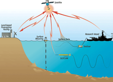
for future predictions. Therefore, modelers need observations to calibrate and verify their models. Unlike atmospheric data sets, oceanic observations have relatively short records and sparse coverage in space. New observing technologies, like satellite remote sensing, acoustic tomography, and the long-lived floats that Ray Schmitt describes in his article inset “ALACE, PALACE, Slocum”, will certainly expand the observing capacity and support climate modeling. A global observational network is likely to be a combination of satellite-borne instruments (which can measure sea surface elevation, wind stress, temperature, and perhaps salinity); automatic instruments, such as buoys and data-transmitting floats; and traditional shipboard instruments. Data collected by these instruments will be sent to a land-based forecasting center, where the most powerful supercomputers will merge current oceanographic data and forecast oceanic conditions for the near future. With the rapid advance of computer technology and our understanding of ocean physics, oceanic forecasting will eventually become a reality—perhaps early in the 21st century, marine and climate forecasting will become routine.
The research discussed in this article was supported by the National Science Foundation and the National Oceanic and Atmospheric Amdinistration’s Global Climate Change Program.
Rui Xin Huang’s primary research interest is large-scale oceanic circulation, including wind-driven gyres and thermohaline circulation. When he was in high school, his dream was to become an inventor like Edison. Through a long and winding road, he came to Woods Hole, and found oceanography an exciting field. He also likes swimming, gardening, and, above all, puzzles and games.
During his graduate student and postdoctoral years, Jiayan Yang was interested mainly in tropical air-sea interaction. He decided to take “a short break” away from the tropics to do a small, high-latitude oceanography project when he was a postdoctoral fellow at the University of California, Los Angeles. He has stayed in high-latitude oceanography ever since. He moved from Los Angeles to New England to get a bit closer to (though still far way from) sea-ice margins. In his leisure time, he likes hiking, swimming, biking, and karaoke.
Slideshow

Slideshow
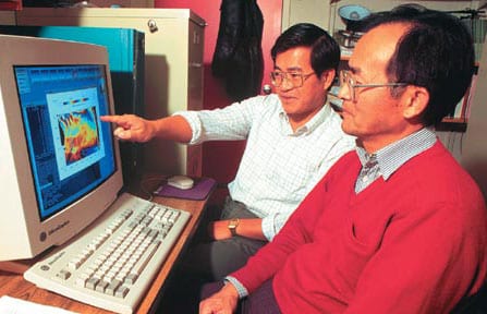
- Authors Rui Xin Huang, right, and Jiayan Yang collaborate on ocean process study and climate prediction models.
- The authors envision a forecasting center that would receive near-real-time data from a variety of sources by satellite transmission for constant updating of ocean climate models. The data sources might include those shown here. The surface mooring transmits meteorological data as well as information from the string of instruments below it. Slocum, described in Schmitt article, surfaces once a week or so at the top of its trajectory to transmit temperature and salinity records from ocean depths, and SeaSoar data on a variety of upper ocean characteristics is beamed from the ship. Data collected by satellites would include sea surface elevation, wind stress, temperature, and perhaps salinity.
Related Articles
- Investigating the ocean’s influence on Australia’s drought
- Extreme Climate
- Warming Ocean Drove Catastrophic Australian Floods
- New Weather-Shifting Climate Cycle Revealed
- Launching the Argo Armada
- A Century of North Atlantic Data Indicates Interdecadal Change
- The El Niño/Southern Oscillation Phenomenon

