|
|
Software - Planview Climatology
Index | BBL | Planview | Xshelf | Cruisetrack
Motivation
The Planview Climatology function is an analysis tool for ocean scientists. With it the user can set up a planview (looking down) grid and compute weighted means and standard deviations of various ocean properties. It operates entirely in the Matlab environment; the
only non-Mathworks products it requires are the m_map
toolbox developed by Rich Pawlowicz and the CSIRO Matlab Seawater Library.
Installation
- Visit the m_map webpage and install this package in its entirety.
Install all
of the GSHHS coastlines. In addition, install
the TerrainBase 5 minute topography. (Rich
provides instructions for installing these databases on the m_map site).
- Download the cl_climo_planview.m m-file.
[Get version 4.0 here].
- Download the latest version of the Seawater toolbox from this CSIRO ftp site.
- Update your Matlab path to reflect the location of these new files.
- At the Matlab command prompt, type help cl_climo_planview to view the help file.
History
 | | |
| Version |
Date |
Changes |
| 5.0 |
08Nov06 |
In addition to some minor bug fixes, the monte-carlo step for computing derivative fields has been replaced by a faster method which calculates the derivative fields during the cast extraction.
|
| 4.0 |
06Jul06 |
An optional quality control module has been added. Due to the (potentially) large number of CTD casts involved, the QC is implemented only as a means to eliminate outliers in temperature and salinity, not analyze individual casts. All calls to the m-file "suptitle" have been eliminated, for better compatibility with Matlab 7.
|
| 3.0 |
24May06 |
In earlier versions, all data--regardless of location--within the vertical range was first extracted and then averaged. In this update, individual CTD casts are first extracted and then a single depth-integrated mean created for each cast. These casts are then fed into the averaging program. This change restores the balance between sparse and well-populated casts. A number of other features, including the ability to print out the figures, has also been added.
|
| 2.0 |
08Nov05 |
Incorporated an iterative search radius to smooth data gaps. Note that this involved changing the order of the input variables.
|
| 1.0 |
29Dec04 |
Initial build.
|
Overview
This program takes a file of unevenly spaced hydrographic
data and creates a planview climatology based on user-specified inputs.
This is Version 3.0, which was tested on Matlab version 7.0 (Release 14, Service pack 1).
function [X, Y, NUMPOINTS, RADIUS, MEANTEMP, STDTEMP, MEANSAL, STDSAL, MEANST, STDST, MEANC, STDC] = cl_climo_planview (filename, season, upperdepth, lowerdepth, gridspacing, Ro, minnumpts, radiusinc, cutoffhighdepth, cutofflowdepth, westbound, eastbound, southbound, northbound, qc, plotyes);
|
 |
The user-defined grid. Range rings are shown in red, extracted data points in green, bathymetry in black.
|
Inputs
filename - specifies name of data file
Data file, in ASCII text format, must have the following columns:
1. Decimal longitude
2. Decimal latitude
3. Year
4. Month
5. Depth (meters)
6. Temperature (C)
7. Salinity (PSU)
Here is a sample file showing how the ASCII structure should look:
Longitude Latitude Year Month Depth Temperature Salinity
-69.000 39.867 1977 12 1.0 18.8198 35.9190
-69.000 39.867 1977 12 5.0 18.7991 35.8020
-69.000 39.867 1977 12 10.1 18.8082 35.9370
-69.000 39.867 1977 12 15.1 18.5573 35.8020
-69.000 39.867 1977 12 20.1 18.5765 35.8180
-69.000 39.867 1977 12 30.2 18.5147 35.8400
-69.000 39.867 1977 12 50.3 18.1313 35.7890
-69.000 39.867 1977 12 75.5 17.3673 35.7010
-69.000 39.867 1977 12 100.6 17.2032 35.6580
-69.000 39.867 1977 12 150.9 14.3676 35.8780
-69.000 39.867 1977 12 402.7 7.6695 35.1580
-69.017 39.917 1951 10 1.0 21.6198 35.4800
-69.017 39.917 1951 10 10.1 22.0480 35.4700
-69.017 39.917 1951 10 24.1 21.6253 35.4900
-69.017 39.917 1951 10 48.3 21.6306 35.4900
-69.017 39.917 1951 10 97.6 16.6340 36.0000
-69.017 39.917 1951 10 195.2 12.9830 35.5900
-69.017 39.917 1951 10 284.9 13.1202 35.5300
-69.017 39.917 1951 10 493.5 12.9011 35.5000....
season - string - is a listing of all seasons (by number) to include in average. For example, Jan & Feb would be '1 2'. Enter 'All' for all.
upperdepth - upper bound (meters) of the climatology.
lowerdepth - maximum depth (meters) of the climatology.
gridspacing - grid spacing in degrees (1/6th degree is 19km lat / 14km lon resolution at 40N).
Ro - Search radius in km (typical is 18km for 0.2 degree grid spacing).
minnumpts - minimum number of data points to use for an average. If this number is not met, a NaN will result for the mean for that grid cell.
radiusinc - Increment that radius will be increased in km to meet minnumpts. If 0, radius will not be iteratively increased. Output nodes that don't have minnumpts observations will be given NaNs.
cutoffhighdepth - Cutoff depth (shallow) - stations with a depth SHALLOWER than this value will be excluded.
cutofflowdepth - Cutoff depth (deep) - stations with a depth DEEPER than this value will be excluded.
westbound - western domain bound - decimal degrees.
eastbound - eastern domain bound - decimal degrees.
southbound - southern domain bound - decimal degrees.
northbound - northern domain bound - decimal degrees.
qc - 0 or 1; 0 will skip the quality control routine and 1 will run it.
plotyes - 0, 1, or 2; 0 will suppress plots, 1 will show plots, and 2 will show plots and save them out as PNG files to the current directory.
Outputs
X - Cross-shelf distance of output grid points in KM (meshgrid format).
Y - Depth of output grid points in M (meshgrid format).
NUMPOINTS - Number of points per output grid node. This, like all of the other output fields, are in the meshgrid format for easy plotting. For example, pcolor(X,Y,NUMPOINTS).
RADIUS - Final search radius in KM.
MEANTEMP - Mean temperature (C).
STDTEMP - Standard deviation of temperature.
MEANSAL - Mean salinity (PSU).
STDSAL - Standard deviation of salinity.
MEANST - Mean sigma-theta (density) (kg/m3) (sigma-theta and sound speed outputs computed using a 1024-realization monte-carlo routine with mean & std temp/salinity as inputs).
STDST - Standard deviation of sigma-theta.
MEANC - Mean sound speed (m/s).
STDC - Standard deviation of sound speed.
 |
|
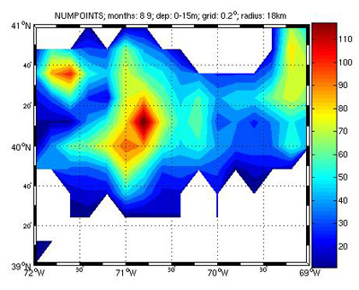
Number of points per grid node for the Nantucket Shoals example.
|
Example 1 - Nantucket Shoals fixed search radius
Given a data file 'ns-all-data.dat', we would like to create a climatology for August
and September near-surface (0 to 15 meters deep) data. The output grid will have 0.2 degree spacing and a search radius
of 18km. For this example, the search radius will be fixed at 18km--any output nodes that do not have 10 realizations (our minnumpts input variable) will be assigned NaNs. Stations shallower than 50m or deeper than 2500m will be excluded.
The study area bounds are 72-69 West, 39-41 North. The quality control routine will be skipped, and the data will be plotted but not printed. The one-line Matlab command to
produce this climatology is:
[X, Y, NUMPOINTS, RADIUS, MEANTEMP, STDTEMP, MEANSAL, STDSAL, MEANST, STDST, MEANC, STDC] = cl_climo_planview('ns-all-data.dat', '8 9', 0, 15, .2, 18, 10, 0, 50, 2500, -72, -69, 39, 41, 0, 1);
Once you have entered that line, the program will begin running. Note that the program expects every parameter to be included, and will crash if the inputs are not there. To repeat, the program will crash if given the wrong number of, or contradictory, inputs (for example cutofflowdepth being deeper than cutoffhighdepth).
The program begins by extracting the chosen seasonal range from the input data. Then, each CTD cast is extracted and derivative variables (sound speed and sigma-t) are computed. The program then decimates all of the points in the desired depth range to a single number using a simple mean. This process ensures that contributions from 1 dBar CTD data do not outweigh CTD casts on a more coarse vertical resolution (such as bottle measurements). The data array is now prepared for the mean field computations.
The first plot the program creates is a setup of your chosen grid parameters. One row and one column of grid points (with corresponding range rings) are plotted. At this point, the program is only plotting the data points that will be averaged. The locations of these points are shown in green. For this test case (grid output figure shown above), notice how there are no points deeper than 2500 meters or shallower than 50 meters. Those data points have already been excluded based on our inputs.
The program then steps through each output grid node, computing the mean and standard deviation for each one. Data points within the range ring for each node are weighted based on their distance from the node center point using a Hamming window filter (Figure 7). Only points within the range ring are included. By changing the size of the range ring, you can control the amount of data overlap (and thus smoothing). A larger range ring will produce smoother output fields, and a smaller range ringnoisier fields. In this example case the range rings are set to a fixed value. If there are not enough points collected within the search radius, NaNs will be assigned to the output fields. In the second example we will look at how a variable search radius changes the fields.
Next the program creates the plots, starting with a plot of the number of points being utilized by each grid node (Figure 6). Note that this will change based on your range ring sizea larger range ring will result in more points per node. Note that this is NOT equivalent to the total number of observations - given that the range ring is a circle, there will always be either overlaps (data points being used for multiple grid nodes) or gaps (data points not being used for any grid nodes).
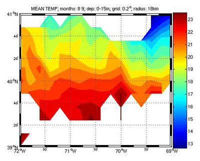
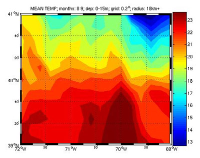
The remaining plots show each of the output fields: mean and standard deviation of temperature, salinity, sigma-t, and sound speed. All of the output fields have the same meshgrid-style array dimensions, and can be plotted simply by using pcolor, contour, etc. X is the longitude array and Y is the latitude. A few output plots are shown below.
 |
|
 |
Sample cl_climo_planview output - mean temperature.
|
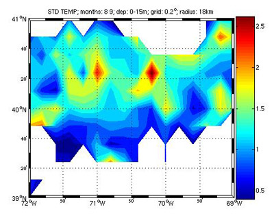
Sample cl_climo_planview output - standard deviation of temperature.
|
Example 2 - Nantucket Shoals variable search radius
Now we would like to modify the above example to fill in the "white space" at the edges. This example is provided to illustrate how the variable search radius feature works. Here is the command to begin the computation--notice that the only change in the syntax for using the variable radius mode is a "10" for radiusinc, instead of "0" in the previous example.
[X, Y, NUMPOINTS, RADIUS, MEANTEMP, STDTEMP, MEANSAL, STDSAL, MEANST, STDST, MEANC, STDC] = cl_climo_planview('ns-all-data.dat', '8 9', 0, 15, .2, 18, 10, 10, 50, 2500, -72, -69, 39, 41, 0, 1);
The variable search radius feature creates an additional while-do loop within the mean computation loop. If the number of points contributing to the mean does not equal minnumpts, then the radius is increased by the chosen step (in this case 10km), and the search is performed again. In this manner the radius continues to increase in 10km increments until minnumpts is reached or exceeded.
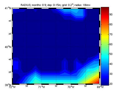
In addition to the plots described above, the program also produces a plot of the final search radius (in km), shown below. Notice how the radius increases to the south, where there were fewer data points present. In the mean temperature plot you can see how the output data is spread into the data poor regions.
 |
|
 |
Sample cl_climo_planview output - variable search radius.
|
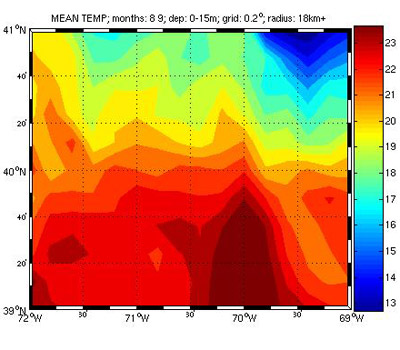
Sample cl_climo_planview output - mean temperature.
|
Example 3 - Nantucket Shoals variable search radius and quality control
The last example is provided to illustrate how the quality control feature works. Here is the command to begin the computation--notice that the only change in the syntax for using the quality control module is a "1" for qc, instead of "0" in the previous example.
[X, Y, NUMPOINTS, RADIUS, MEANTEMP, STDTEMP, MEANSAL, STDSAL, MEANST, STDST, MEANC, STDC] = cl_climo_planview('ns-all-data.dat', '8 9', 0, 15, .2, 18, 10, 10, 50, 2500, -72, -69, 39, 41, 1, 1);
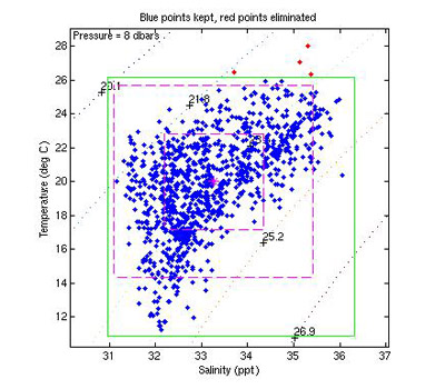
The quality control module works by creating an extra figure (shown below, left). After the correct months have been extracted and the points averaged over the selected depth range, they are plotted on a temperature-salinity plot. Note that this T-S plot is different from the standard T-S plot in that the points are all from the same depth. Since we are not comparing deep points with shallow points, outliers are much easier to pick out. The user is prompted to pick the upper left and lower right corners of a box that will enclose the "good" points. After choosing the box, the program will exclude the out-of-range points and proceed as before. A sample mean temperature output is shown below (right).
 |
|
 |
Sample cl_climo_planview output - quality control summary.
|
Sample cl_climo_planview output - mean temperature.
|
|