Sample bottom boundary layer ATC output.

This suite of Matlab m-files computes the accumulated property change (APC) (property being potential temperature, salinity, or spiciness) along isopycnals in a 2-D CTD section across an area of steeply sloping topography (see sample output at right). The final output is an interpolated, regularly gridded section of APC. The method and applications of the software are explained in the Linder et al. 2004 JGR paper on detaching bottom boundary layers. Through a user-friendly GUI or a single Matlab function, the user has complete control over the many variables. It operates entirely in the Matlab environment; the only non-Mathworks products it requires are the CSIRO Seawater toolbox, spice.m, suptitle.m, and Matlab interpolation software coded by WHOI's Roger Goldsmith. This code is adapted from software written by Bob Pickart. The rationale behind this methodology is explained in detail in this Pickart 2000 JPO paper.

Installation:

• Visit the CSIRO SEAWATER webpage and install this package in its entirety.
• Download and unpack this Matlab interpolation software written by Roger Goldsmith.
• Download and unpack this zip file, which contains the BBL m-files, spice.m, suptitle.m, and two practice data files.
• Update your Matlab path to reflect the location of these new files.
• Modify the default path (bbldirectory) in cl_bblini.m.
• At the Matlab command prompt, type cl_bblgui. This will launch the GUI. For advanced users who will be running the program as part of another program, there is also a functional form- type help cl_bblfcn for usage.

History:

Version	Date	Changes
1.2	10Oct05	- Added cl_bblfcn.m, which allows you to compute accumulated property fields with one Matlab function call - Fixed bug that caused program to crash if smoothing was set to 0. A value of 0 will now bypass smoothing routines. - Combined two plots into new plot 2, which better shows the chosen and rejected contours.
1.1	26Sep05	Comprehensive overhaul
1.0	18Apr02	Inital build

Overview - GUI form

Type cl_bblgui at the Matlab prompt. The BBL GUI should appear (shown above). Note that it is composed of several different "windows" and buttons. This description will proceed in order of the way the program should be used. This overview will start at the upper left, work down the left column, and then down the right hand side column from top to bottom.

The first entry is an option to change your path. This is where the program will look for the data files. If the path is not set correctly, a warning button will appear alerting you to change your directory. Under the path entry box are several buttons. From left to right, the buttons will clear all figure windows "Clear figs", save your default entries in the GUI "Save defaults", create a pop-up window with program information "About", and exit the GUI "Exit".

The next radio button allows you to pick the parameter you would like to "accumulate". The three choices are temperature, salinity, and "spiciness", a derived value that is orthogonal to density. The final button on the left hand side is the option to save out the variables after the program is done running. All of the program variables are saved to a Matlab mat-file named outfile.mat.

There are three Help buttons located on the GUI. Pushing these buttons will give you specific tips for each of the corresponding "windows."

Preparing the input data - GUI form

There are some restrictions regarding file format. The program expects the following format (and will crash if format not followed!)
- Input file: a Matlab .mat file containing these arrays:
One six-column array named "posits"
1: Station number (1 through Numstations)
2: Latitude degrees (- for South)
3: Latitude decimal minutes (- for South)
4: Longitude degrees (- for West)
5: Longitude decimal minutes (- for West)
6: Bottom depth of cast (meters)

One array for each station named "rawprofileX" where X is the station number from the posits array - each is a 3 column array
1: Pressure (dbar)
2: Temperature (C) - NOT potential temperature, that will be computed later
3: Salinity

Looking at an example (a February 1984 CTD section from the SEEP program), you can see the variables that need to be in the matlab mat-file. The number of rows in the posits array must be the same number as the number of raw profiles. Note that if you don't want to use the degrees / decimal minutes convention, you can simply use decimal degrees and leave minutes as columns of zeroes. Note also that rawprofile1 is assumed to be the most onshore profile, and that the profiles will get progressively deeper.

Running the program and interpreting the results

The hardest part in running the program is setting up your data files. Once those are properly configured and the GUI has the correct plotting parameters, just hit the Compute/Plot button. The program will immediately begin running. In this section I will discuss the sample output figures. Runtime is approximately 6 minutes on my machine running this sample case.

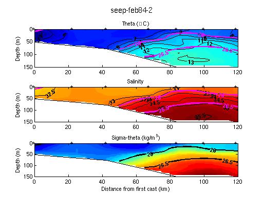Plot 1. Contoured potential temperature, salinity, and potential density (with potential density overlaid in magenta on the top two plots). The program first creates an evenly spaced grid of potential temperature, salinity, and potential density from the (most likely) unevenly spaced raw CTD profiles. Potential temperature (theta) and potential density (sigma-theta- reference level 0 dbars) are computed from the T, S, and P input data.

Plot 2. Potential density contours. This plot shows both the contours that the program is NOT using (black) and the ones that it will use in the integration (magenta). In the case of the chosen contours, green dots indicate the start of the line segment, and red dots indicate the end points. The program has eliminated contour segments that a) start AND end at the surface, b) are closed loops, c) start AND end on the bottom, d) start from LHS of page, and e) start from the BOTTOM of page. We are ultimately left with contours that start on the seafloor (indicated by the black line on this plot) and end either at the surface or the RHS of the plot.

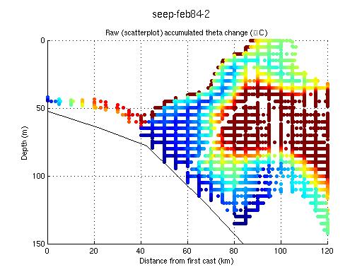Plot 3. This is a scatter plot of the accumulated property (in this case potential temperature). Essentially this is the raw output. The program has integrated along the contours shown in Plot 3, assuming a starting value of zero at the seafloor.

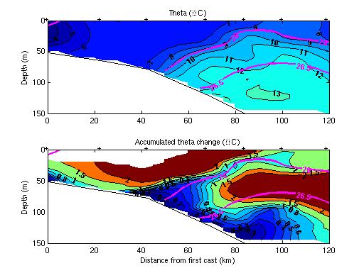Plot 4. The top plot is the potential temperature (in color) with potential density overlaid as magenta contours (same as Plot 1A) and the bottom is the accumulated property (in this case potential temperature) with potential density overlaid as magenta contours. Note the plume of low-ATC rising up from the x=50km, y=-75m point on the seafloor along the 26.0 isopycnal.

Now you have four plots taking you through the entire analysis process... The final plot essentially shows you how your chosen property (theta, salinity, or spiciness) is changing along isopycnals that have originated on the seafloor and terminate at the surface or offshore edge of the plot. We believe that a minimum in accumulated theta (such as the blue-colored plume in the above example) is indicative of bottom boundary layer detachment along that isopycnal.

The functional form

Certain users, for example those who work with regular grids instead of unevenly spaced data, may prefer the functional form. This one m-file allows you to bypass the GUI environment completely. Since this is a Matlab function, none of the extraneous intermediate variables will clutter your workspace. Best of all, it can be run within existing programs, making it possible to compute APC for as many sections as you want with complete automation.

The major difference between this code and the GUI code is the format for the input data. The program assumes that instead of supplying unevenly spaced CTD casts, as in the GUI version, you will provide regularly gridded fields of X, Y, potential temperature/salinity/spiciness, and potential density. The output array, APC, is the accumulated property change forced onto the same regular grid that the user supplied with the input data. To see a sample of the input arrays that are required, load the provided sample data file by typing load seep-feb84-2-FCN.

The program is called using this syntax:
APC=cl_bblfcn(origRegX,origRegY,RegProperty,RegSigmatheta,avgsec,parameter,deltasigma,smoothing,plotyes,apccontours,apcaxis,denscontours);

Inputs:
origRegX - A regularly gridded array (Matlab meshgrid format) of the x-position of the property & density data (km)
origRegY - A regularly gridded array (Matlab meshgrid format) of the y-position of the property & density data (m)
RegProperty - A regularly gridded array of potential temperature (or salinity or spiciness depending on what you want to "accumulate") in the Matlab meshgrid format
RegSigmatheta - A regularly gridded array of potential density in the Matlab meshgrid format ** please use sigma-theta minus 1000 kg/m^3; i.e. data in the range 23-29, instead of 1026-1029...
avgsec - Bottom profile - a two column array of values - first column is the x-distance (km) and the second column is the depth (m). Depth should be given as negative numbers.
parameter - Use 1 for theta, 2 for salinity, and 3 for spiciness--note that this only affects labeling
deltasigma - Interpolation step. Smaller number means more accuracy at the cost of more computation time. 0.05 is typical.
smoothing - how much the data is smoothed when using ppzgrid. A value of 2 is fairly typical.
plotyes - 0 or 1. 0 will suppress plots. 1 will show plots.
apccontours - these are the contours overlaid on the final plot. Use array of values - see example below
apcaxis - An array of two numbers, such as [0 2], which will determine the color range of the final accumulated property change plot
denscontours - these are the density contours overlaid in magenta on the final plot. Use array of values- see example below

Example: Middle Atlantic Bight test case - SEEP February 1984 section
APC=cl_bblfcn(origRegX,origRegY,RegTheta,RegSigmatheta,avgsec,1,0.05,2,1,[0 0.1 0.2 0.3 0.4 0.5 0.6 0.8 1 1.5 2],[0 2],[25 25.5 26 26.5 27 27.5]);

Given input arrays origRegX, origRegY, RegProperty, RegSigmatheta, and avgsec, the program will compute accumulated POTENTIAL TEMPERATURE change (parameter=1), with a deltasigma step of 0.05 kg/m³, smoothing of 2, and will show three output plots (the same plots as 2, 3, and 4 shown above). The APC will be contoured on these values: 0, .1, .2, .3, .4, .5, .6, .8. 1, 1.5, 2 and the color range of the final output plot will be from 0 to 2 Celcius. Potential density contours will be overlaid in magenta at the following values: 25 25.5 26 26.5 27 27.5. The output array is named APC; the X and Y posits of the final values are prescribed by origRegX and origRegY (the original regularly gridded distance and depth arrays).