|
Preliminary Results
Model Details
We use the fully optimized and paralellized code
developed by Dr. Kraig Winters at the University of Seattle,
Washington. The model solves the three-dimensional f-plane
Boussinesq equations, coupled with an advection-diffusion equation
for the density using a semi-/pseudo-spectral approach.
Preliminary runs are conducted using either 64x64 or 128x128
gridpoints in the horizontal, and 64 gridpoints in the vertical, and
a dimensionful domain size of Lx=Ly=500m,
and Lz=50 m. In order to keep computations logistically
tractable, we artificially elevate the value of the Coriolis term,
f, by a factor of 10. This serves to reduce the ratio of
the buoyancy frequency to the Coriolis frequency, N/f, and
thus allows us to capture the dynamics associated with each of these
time scales without having to perform prohibitively long numerical
integrations. The artificially low ratio of N/f (order 10
vs. typical values of order 100) does not alter the inherent
dynamics of the system.
Spinup
The model is spun up to a statistically steady state by injecting
stratification anomalies periodically but at random locations in the
domain, and allowing the system to adjust dynamically. The effect of
this is to provide a quasi-steady source of potential energy (PE)
to the system, which is then converted to kinetic energy (KE)
through a combination of cyclostrophic, geostrophic, and/or
frictional adjustment. A statisctically steady state is reached
when the rate of energy input is balance by energy dissipation at
the smallest scales.
The anomalies are generated by imposing a spatially varying diapycnal
diffusivity which is localized in both the horizontal and vertical
according to a pre-determined Gaussian profile,
When applied to a linear density profile, this creates a gaussian
density anomaly of the form,
where x- and y-dependence in the latter expression are
implied. Typical stratification anomaly and diffusivity profiles
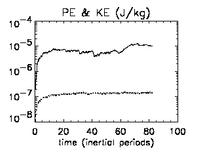
are shown in Figure 1. An example of the evolution of PE and KE
during spinup is shown in Figure 2.
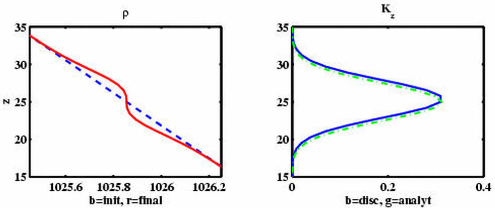
Figure 1. Gaussian density anomaly and diffusivity profiles
used in numerical simulations.
|
|
Figure 2. Time series of potential and kinetic energy showing
model spinup and equilibration.
|
|
Once the model reaches a statistically stationary state, we release
a passive tracer into the flow.
Subsequently, as additional density anomalies are introduced into
the system, the diffusivity profile applied to density is also
applied simultaneously to the Lagrangian tracer field.
Results
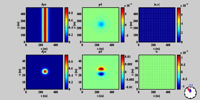
Figure 3 shows the results of a simulation in which a single
density anomaly was released at the center of the domain. At the
same time as the anomaly was introduced, a streak of tracer of the
same width and vertical scale was also introduced.
The result shows the effect of a single anomaly displacing the
tracer. The initial radial displacement of tracer
combined with the anti-cyclonic rotational displacement of the
patch are evident in the animation. Corresponding density and
velocity fields are also shown. Total simulation time was
approximately 6 inertial periods.
|
|
(Click on image to view mpeg animation - 7.7 Mbyte.)
|
|
Figure 3. Model run using a single density anomaly at the
center of the domain. Top panels are plan views of dye,
potential density anomaly, and horizontal velocity. Bottom
panels are vertical cross sections of the same variables.
|
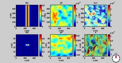
Figure 4 shows the results for a simulation in the case of a fully
spun field of random stratification anomalies. Again the tracer
was injected as a single streak of the same width and vertical scale
as the density anomalies. The result shows the stirring effects of
a random field of anomalies on the tracer.
Corresponding density and velocity fields are also shown.
Total simulation time in this case was approximately 37 inertial periods.
|
|
(Click on image to view mpeg animation - 9.7 Mbyte.)
|
|
Figure 4. Model run using a field of random density anomalies
distributed throughout the domain. Top panels are plan views of
dye, potential density anomaly, and horizontal velocity. Bottom
panels are vertical cross sections of the same variables.
|
The above simulations provide a means of evaluating the effective
lateral dispersion caused by the relaxation of diapycnal mixing
events. Theoretical predictions based on scaling of the horizontal
momentum equations (Sundermeyer, 1998) suggest that the horizontal
diffusivity due to such stirring should scale approximately as,
where DN, h, and L are
the change in buoyancy frequency, the half-height, and the horizontal
scale of the anomaly, respectively; U is a velocity scale
associated with the adjustment, and R is the deformation
radius associated with the anomaly, and
n is the frequency at which
anomalies occur.
Preliminary results using a relatively modest model resolution of
643 gridpoints indicate that the above parameter dependence
is approximately valid to lowest order. Specifically, we have found
that compared to a base run, increasing the buoyancy frequency
N2 by a factor of 2 increases
the effective horizontal diffusivity
Kh
by a factor of 3. Similarly, increasing the rate of anomaly input
by a factor of 2 increases
Kh
by a factor of 1.5. Finally, increasing the height of the anomalies,
h by a factor of 2 increeases
Kh
by a factor of 20. (Note that the expected dependence of
Kh
on the above parameters is best seen in the first equality of the
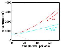
above expression.) Horizontal diffusivity estimates based on the
time rate of change of the horizontal second moment of tracer for
the above described simulations are shown in Figure 5.
|
Increasing N2
by a factor of 2 increases
Kh
by a factor of 3.
|
|
|
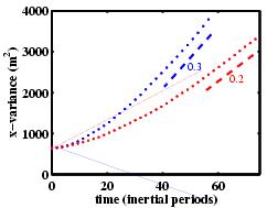
Doubling the rate of anomaly input increases
Kh
by a factor of 1.5.
|
|
|
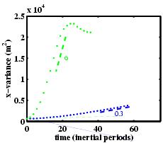
Doubling the height of anomalies increases
Kh
by a factor of 20.
|
|
|
Figure 5. Time series of the second moment of tracer used
to test theoretical parameter dependence. Horizontal
diffusivities are estimated based on the slope of the curves
during the linear growth phase of the tracer moments.
|
(... More results coming soon - as time permits!)
|