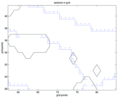
Sections to be analyzed by PAGO are either listed in PAGO function define_section (and further saved in .mat file, to be given to PAGO function sections_MODEL) or manually defined by the user (within sections_MODEL). We recommend to use define_section if the section is to be used in various grids. A pre-defined set of sections for the North Atlantic (sections_NA.mat) and the global ocean (sections_GL.mat) are available in define_section. Make sure that the grid subset is compatible with the section locations.

End points and corners of sections are defined by their longitude and latitude, so that the definition is the same for all grids. For each segment of each section, the positive direction for the normal transport must be defined using a two-letter code (NE, NW, SE or SW), each letter referring to the direction (North, South, East or West) in the grid space. In order to ensure that the normal transport is properly defined, PAGO function sections_MODEL produces a figure with all sections and dots - one dot for each grid face followed by the sections (figure 12). Dots may be viewed as the head of arrows normal to the section heading in the direction defined as positive for the volume transport. Hence the definition of the positive normal transport is ok if all the dots are located on the same "side" of the section (see figure below). Depending on this definition, u and v velocities may be multiplied by -1 before being saved as normal velocities in PAGO functions loaddata_*.

When using the default grid subset and sections for the North Atlantic, it is recommended to use built-in corrections in sections_MODEL. Otherwise, make sure that the location of section end points and corners, as well as directions, is suitable for the analysis. Several questions are asked when running sections_MODEL to make sure that the definition of section s is ok. For example, as most sections are expected to go from coastline to coastline, the program will ask for user confirmation in case the end point of a section is not in land. This may happen for the sections defined from Iceland to Faroe's Islands and from Faroe's Islands to Scotland, as Faroe's Islands are missing in most climate models. It is not a problem, for the rest of the programs, if the end point of a section is in water.

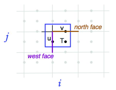
We assume that the dataset gives temperature and salinity at the center of the grid cell, and velocity (if available) either at the corners or at the center of the grid faces. In PAGO functions loaddata_*, this information is interpolated and remapped so that temperature, salinity and velocities are available at the center of the western and northern grid faces (see figure below). Temperature and salinity are averaged from the centers of the 2 adjacent grid cells to the center of the grid faces, taking into account missing values in land (but no grid scale factor is taken into account in this process). In case of C-grid data, no interpolation is required for the velocities (see loaddata_IPSL for example). In case of B-grid data, the volume transport at the corner of the grid cells is computed and then split in 2 to the center of each adjacent faces (see loaddata_CCSM for example). Data information loaded along sections, i.e. temperature, salinity and velocity, can be mapped using PAGO function figure_section_1l.

Various indices describing the transport across sections are calculated in PAGO function indices_MODEL. Definition and units are specified in the netCDF files. These indices concern the transport of volume (in Sv), heat (in PW), salt (in psu*Sv) and freshwater (mSv). Freshwater is referenced to the average salinity of the Arctic (34.8) but this definition may be changed in indices_MODEL directly. There is no interpolation of the data on the vertical, whatsoever.

PAGO indices include time series, that can be saved in netCDF format (see output page):

• (i) the net transports, i.e. the integral of normal velocities eventually multiplied tracers.
• (ii) the total transports of tracers when assuming no net volume transport across the section. This quantity is particularly relevant when comparing with observation estimates built on the same assumption.
• (iii) the overturning components in z vertical coordinates. For volume transport, the first maximum from the surface is given as well as the depth of this maximum. The net transports are systematically removed prior to calculating the overturning components. The overturning component of tracer transports is defined as the product of the overturning component of velocity and tracer profiles, calculated separately.
• (iv) the overturning components in density coordinates, similarly to z-vertical coordinates except that velocities and tracers are binned into density vectors. Four different density vectors are available: *_s0_1 uses potential density referenced to the surface, *_s0_2 as well but with twice as much resolution as *_s0_1, *_s1 uses potential density referenced to 1000 dbar, and *_s2 uses potential density referenced to 2000 dbar. Density may be calculated using two different equations of state (see comments in indices_MODEL).
• (v) the barotropic and baroclinic components, the latter being the residual of the total transports, overturning and barotropic components.
• (vi) transports integrated over fixed vertical intervals. The limits of those intervals, defined in indices_MODEL, is fixed but their actual depth depends on the depth of the data levels as there is no vertical interpolation of the data.
• (vii) transports integrated over fixed density intervals, to be defined by user when running indices_MODEL.

More indices are produced by indices_MODEL. All indices are split in two categories: simple diagnostics, which require minimum calculations ( such as time series of type i, ii and iii), and full diagnostics (all indices). User has to specify, when running indices_MODEL, which sections to be considered for simple and full diagnostics.