|
|
Software - Xshelf Climatology
Index | BBL | Planview | Xshelf | Cruisetrack
Motivation
The Xshelf Climatology function is a Matlab analysis tool for ocean scientists. With it the user can assimilate historical data in a given study area into a single cross-shelf (looking "sideways" through the water column) transect. The program was developed to analyze areas of steeply sloping topography such as the Middle Atlantic Bight (MAB) shelfbreak. In a dynamic, topographically influenced environment like the MAB shelfbreak, traditional spatial climatologies can eliminate strong gradients by averaging together shelf and slope water parcels. This program assumes that along-shelf gradients are minimal compared to cross-shelf gradients.
Two-dimensional high-resolution maps of the means and standard deviations of various ocean properties are computed. Using a user-selectable baseline isobath, the program creates a new bathymetry-following coordinate system. This is the key feature of the program - by segregating shallow and deep water parcels, the program aims to preserve the cross-shelf gradients. It operates entirely in the Matlab environment; the
only non-Mathworks products it requires are the m_map
toolbox developed by Rich Pawlowicz, the CSIRO Seawater toolbox, and the function cl_montecarlo.m. In addition, if you would like smoothed and extrapolated output, you will need to download Roger Goldsmith's adaptation of the PlotPlus ppzgrid software (all Matlab m-files). Smoothing is optional--if you don't want smoothed output you don't need to download this toolbox. Note that this code was built and tested using Matlab version 7--you may encounter problems with earlier versions.
Installation
- Visit the m_map webpage and install this package in its entirety.
Install all
of the GSHHS coastlines. In addition, install
the TerrainBase 5 minute topography. (Rich
provides instructions for installing these databases on the m_map site).
- Download the cl_climo_xshelf.m m-file.
[Get latest version here for Matlab 7].
- Download the latest version of the Seawater toolbox from this CSIRO ftp site.
- Download Roger Goldsmith's zipped ppzgrid files.
- Update your Matlab path to reflect the location of these new files.
- At the Matlab command prompt, type help cl_climo_xshelf to view the help file.
History
 |
|
|
| Version |
Date |
Changes |
| 4.0 |
11Oct06 |
Major change to methodology--sigma-t and sound speed are now computed as each cast is ingested from the input file, so the Monte-Carlo step has been eliminated. This results in more accurate mean and standard deviations of these variables. The program also eliminates duplicate casts, and prints a summary of cast statistics in the Matlab command window at the end of the run. |
| 3.0 |
24May06 |
Output variables AVGSEC and BASELINE added. A number of other small bugs have been fixed, and the documentation has been improved. |
| 2.1 |
5Apr06 |
Code updated to exclude casts outside the precise study area box limits. |
| 2.0 |
20Mar06 |
Each input cast now interpolated to user-selected vertical resolution before averaging. New code added for QC, decimation by cross-shelf bin, and automated plot saving. |
| 1.1 |
9Mar05 |
A number of small bugs fixed. |
| 1.0 |
29Dec04 |
Initial build.
|
Overview
This program takes a file of unevenly spaced hydrographic
data and creates a cross-shelf climatology based on user-specified inputs.
function [X,Y,AVGSEC,BASELINE,NUMPOINTS,MEANTEMP,STDTEMP,MEANSAL,STDSAL,MEANST,STDST,MEANC,STDC] = cl_climo_xshelf(filename, season, bathyline, bathychoice, maxdepth, onshore, offshore, hbinsize, vbinsize, westbound, eastbound, southbound, northbound, minnumpts, qc, decimate, smoothing, plotyes);
|
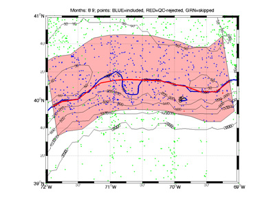 |
The user-defined study area. Bathymetry lines are shown in black, the baseline isobath (in this case 100 meters) shown in dark blue, and data points shown in blue (note that QC-rejected points are shown in red and out-of-bounds points in green). In this example, the user has already chosen the new baseline, which is shown as a red line. The light red shaded box is the approximate area that will comprise the final average - in this case 60km onshore and 40km offshore, measured perpendicular to the user-defined baseline.
|
|
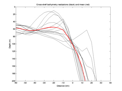 |
After the user selects the new baseline, the program shows the user the individual cross-shelf bathymetry profiles, and the mean profile that will be used for the output.
|
Inputs
filename - specifies name of data file
Data file, in ASCII text format, must have the following columns:
1. Decimal longitude
2. Decimal latitude
3. Year
4. Month
5. Depth (meters)
6. Temperature (C)
7. Salinity (PSU)
Here is a sample file showing how the ASCII structure should look:
Longitude Latitude Year Month Depth Temperature Salinity
-69.000 39.867 1977 12 1.0 18.8198 35.9190
-69.000 39.867 1977 12 5.0 18.7991 35.8020
-69.000 39.867 1977 12 10.1 18.8082 35.9370
-69.000 39.867 1977 12 15.1 18.5573 35.8020
-69.000 39.867 1977 12 20.1 18.5765 35.8180
-69.000 39.867 1977 12 30.2 18.5147 35.8400
-69.000 39.867 1977 12 50.3 18.1313 35.7890
-69.000 39.867 1977 12 75.5 17.3673 35.7010
-69.000 39.867 1977 12 100.6 17.2032 35.6580
-69.000 39.867 1977 12 150.9 14.3676 35.8780
-69.000 39.867 1977 12 402.7 7.6695 35.1580
-69.017 39.917 1951 10 1.0 21.6198 35.4800
-69.017 39.917 1951 10 10.1 22.0480 35.4700
-69.017 39.917 1951 10 24.1 21.6253 35.4900
-69.017 39.917 1951 10 48.3 21.6306 35.4900
-69.017 39.917 1951 10 97.6 16.6340 36.0000
-69.017 39.917 1951 10 195.2 12.9830 35.5900
-69.017 39.917 1951 10 284.9 13.1202 35.5300
-69.017 39.917 1951 10 493.5 12.9011 35.5000....
season - string - is a listing of all seasons (by number) to include in average. For example, Jan & Feb would be '1 2'. Enter 'All' for all.
bathyline - baseline isobath for the climatology in meters.
bathychoice - either 0, which forces the user to hand-pick the baseline, or a 2 column array of lon/lat pairs defining the baseline, which bypasses the baseline chooser routine.
maxdepth - maximum depth of the climatology in meters.
onshore - extent of onshore domain in kilometers.
offshore - extent of offshore domain in kilometers.
hbinsize - horizontal bin size in kilometers.
vbinsize - vertical bin size in meters.
westbound - western domain bound in decimal degrees.
eastbound - eastern domain bound in decimal degrees.
southbound - southern domain bound in decimal degrees.
northbound - northern domain bound in decimal degrees.
minnumpts - minimum number of data points to use for an average. If this number is not met, a NaN will result for the mean for that grid cell.
qc - 0 or 1; 0 will skip the quality control routine and 1 will run it.
decimate - 0 or 1; 0 will bypass decimation routine and 1 will run it.
smoothing - smoothing applied by ppzgrid routine. A value if 2 is typical for hydrographic section data. Enter 0 to bypass smoothing.
plotyes - 0, 1, or 2; 0 will suppress plots, 1 will show plots, and 2 will show plots and save them out as PNG image files to the current directory.
Outputs
X - Cross-shelf distance of output grid points in KM (meshgrid format).
Y - Depth of output grid points in M (meshgrid format).
AVGSEC - 2-column file defining the average cross-shelf bathymetry profile. The first column is distance in KM and the second is depth in M.
BASELINE - 2-column file of the user-selected baseline. This is preserved as an output variable so that for future runs, you can use this variable as an INPUT-see bathychoice, above.
NUMPOINTS - Number of points per output grid node. This, like all of the other output fields, are in the meshgrid format for easy plotting. For example, pcolor(X,Y,NUMPOINTS).
MEANTEMP - Mean temperature (C).
STDTEMP - Standard deviation of temperature.
MEANSAL - Mean salinity (PSU).
STDSAL - Standard deviation of salinity.
MEANST - Mean sigma-theta (density) (kg/m3) (sigma-theta and sound speed outputs computed using a 1024-realization monte-carlo routine with mean & std temp/salinity as inputs).
STDST - Standard deviation of sigma-theta.
MEANC - Mean sound speed (m/s).
STDC - Standard deviation of sound speed.
 |
|
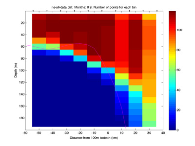
Number of points per grid node for the Nantucket Shoals example.
|
Example - Nantucket Shoals
Given a data file 'ns-all-data.dat', we would like to create a cross-shelf climatology for August
and September data along a baseline isobath of 100m (user must choose the baseline by hand). The output fields will extend from 60km
onshore to 40km offshore and 200m in depth. The vertical bin size is 10 meters
and the horizontal bin size is 10km. The study area bounds are 72-69
West, 39-41 North.
A minimum of 10 realizations must be present to make a mean, the quality control and decimation routines will be run, a factor of
2 smoothing will be applied to the results, and the data will be plotted but the plots will not be saved.
The one-line Matlab command to
produce this climatology is:
[X, Y, AVGSEC, BASELINE, NUMPOINTS, MEANTEMP, STDTEMP, MEANSAL, STDSAL, MEANST, STDST, MEANC, STDC]=cl_climo_xshelf('ns-all-data.dat', '8 9', 100, 0, 200, 60, 40, 10, 10, -72, -69, 39, 41, 10, 1, 1, 2, 1);
Once you have entered that line and hit return, the program will begin running. Note that the program expects every parameter to be included, and will crash if the inputs are not there. To repeat, the program will crash if given the wrong number of, or contradictory, inputs (for example westbound being greater than eastbound). There is a very minimal amount of error checking built into the code.
The program will first plot the study area, with the chosen baseline isobath plotted as a dark blue line (shown in the figure above). Since the 'bathyline' parameter was 0, the user, using the left mouse button, must select a new baseline. This baseline is critical to the program - it is used to define the bathymetry-following coordinate system. Note also that no points beyond the edges of your line will be included, so this can be used to extract a specific geographic subset of your domain. Once you are finished, click the right mouse button and the program will continue (note that your Lon/Lat choices will be saved into array BASELINE). The user can instead enter a 2-column array of Lon/Lat pairs defining the baseline to bypass this stage. This is especially useful when running the program multiple times for different time periods--both in terms of saving time and ensuring consistent results.
The program then extracts the casts from the data file, sorts them into cross-shelf bins, computes the derivative variables, and interpolates the cast data onto the vertical bin depths. The program assumes that for each cast, the year, month, latitude, and longitude are identical, and the depth is increasing. If any one of these criteria fails, then it is assumed that a new cast has begun. After each cast is extracted, its perpendicular distance to the baseline is computed. Based on this distance, a cross-shelf bin number is assigned. Then, the derivative variables of sigma-t and sound speed are calculated. All of the cast variables (temperature, salinity, sigma-t, and sound speed) are then interpolated (using the Matlab interp1 function) onto the user-selected vertical bin depths. The process is repeated until all of the casts are extracted (the total number of casts is displayed in the command window). The output values are stored in a single regular array. This phase is the most computationally intensive part of the program.
After this is complete, the program looks for duplicate casts and eliminates those.
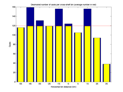
Next the program creates two plots showing the distribution of data points. The first plot is a histogram showing how the data is distributed throughout the cross-shelf bins. The next plot is much more descriptive, showing the number of points contributing to each bin. Obviously, this will change based on your chosen horizontal and vertical bin sizes.
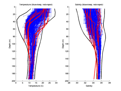
Next, the program enters the quality control (QC) and decimation stages (note that these steps can be bypassed by using an input parameter of 0). The QC is accomplished through an iterative process. The user is first shown all of the cast T/S profiles in blue, plus the mean and standard deviation envelope in black. Next, the user will choose a multiple of the standard deviation envelope -- casts within this envelope will be kept, and those outside will be flagged. If the temperature OR salinity is outside the envelope at any depth point in the profile, the entire cast will be flagged as questionable. The flagged casts will be plotted in red. The user will then be given the opportunity to accept this decision. If not satisfied, you will start the process over. After this initial flag decision, the user will be asked to review each cast for inclusion/exclusion. At this point the user can choose to accept or reject individual casts. The figure below left shows an example of casts that were eliminated by choosing a 3.5* standard deviation envelope and eliminating all of those (16) casts.
The next phase is decimation. The goal in this step is to reduce casts in horizontal bins with too many (relative to the other bins) casts. First, the mean number of casts for each bin is computed. Then, the bins with more casts than this number will be sorted on julian date, and casts eliminated evenly in time to achieve the mean number of casts. For this example (see figure below, right), the mean number of casts among the cross-shelf bins is 120. Data from five of the bins was eliminated in order to reduce oversampling biases.
 |
|
 |
Sample quality control results.
|
Sample cast decimation results.
|
The program then begins to compute the means and standard deviations of temperature, salinity, sigma-t, and sound speed for each output grid node. No weighting is assigned to the points - they are simply binned, and mean and standard deviation are computed for each bin. After these computations, if the user has specified a smoothing amount, the fields will be regridded (extrapolating the data if necessary) and smoothed.
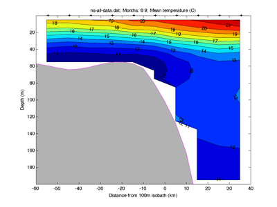
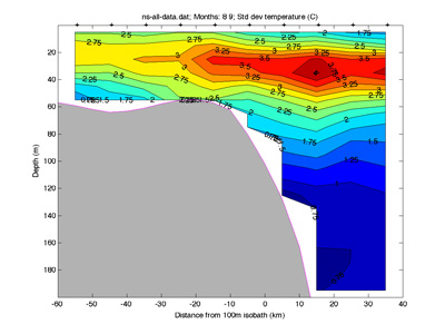
After performing the computations, the program will (if the user chooses) plot each of the output fields: mean and standard deviation of temperature, salinity, sigma-t, and sound speed. All of the output fields have the same meshgrid-style array dimensions, and can be plotted simply by using pcolor, contour, etc (e.g. pcolor(X,Y,MEANTEMP); ). X is the longitude and Y is the latitude. Two output plots (mean and standard deviation of temperature) are shown below.
 |
|
 |
Sample cl_climo_xshelf output - mean temperature.
|
Sample cl_climo_xshelf output - standard deviation of temperature.
|
|