|
|
 |
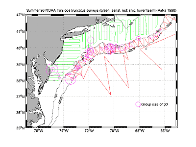 |
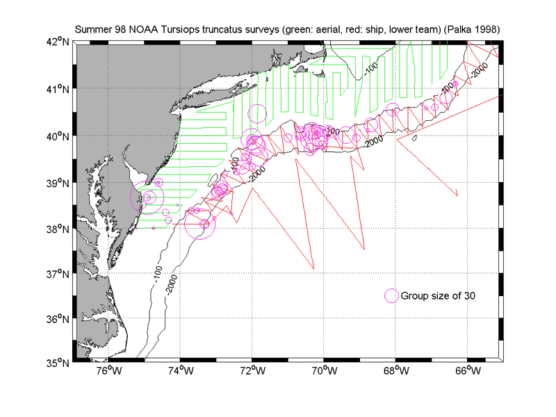
NOAA summer 1998 Tursiops truncatus
surveys (data courtesy Debbie Palka, NOAA). [click
to enlarge]
|
Science - Correlation of bottlenose dolphin positions with the shelfbreak front
<< back
to science index
Collaborators
Glen Gawarkiewicz (WHOI), Debbie Palka (NOAA), and Gordon Waring (NOAA)
Background
A great deal of effort has recently been directed toward defining habitats for marine mammals. Concerns over human-generated sound in the ocean, the status of endangered species, and the increasing pressures of human development along the coast make this a timely issue. Bottlenose dolphin (Tursiops truncatus) sightings taken from a survey in July/August, 1998 are used to examine the distribution of the dolphins relative to the bathymetry and the position of the shelfbreak front. There is a peak in abundance at the 100 m isobath, which corresponds to the mean position of the foot of the shelfbreak front. 95% of the sightings in our study region were within the climatological mean position of the front. The distribution is limited by sub-surface salinity gradients within the front and not sea surface temperature, which is commonly used to define marine mammal habitat. We conclude that the foot of the front is an important "hotspot" for the presence of bottlenose dolphins and possibly other marine mammals.
Plots
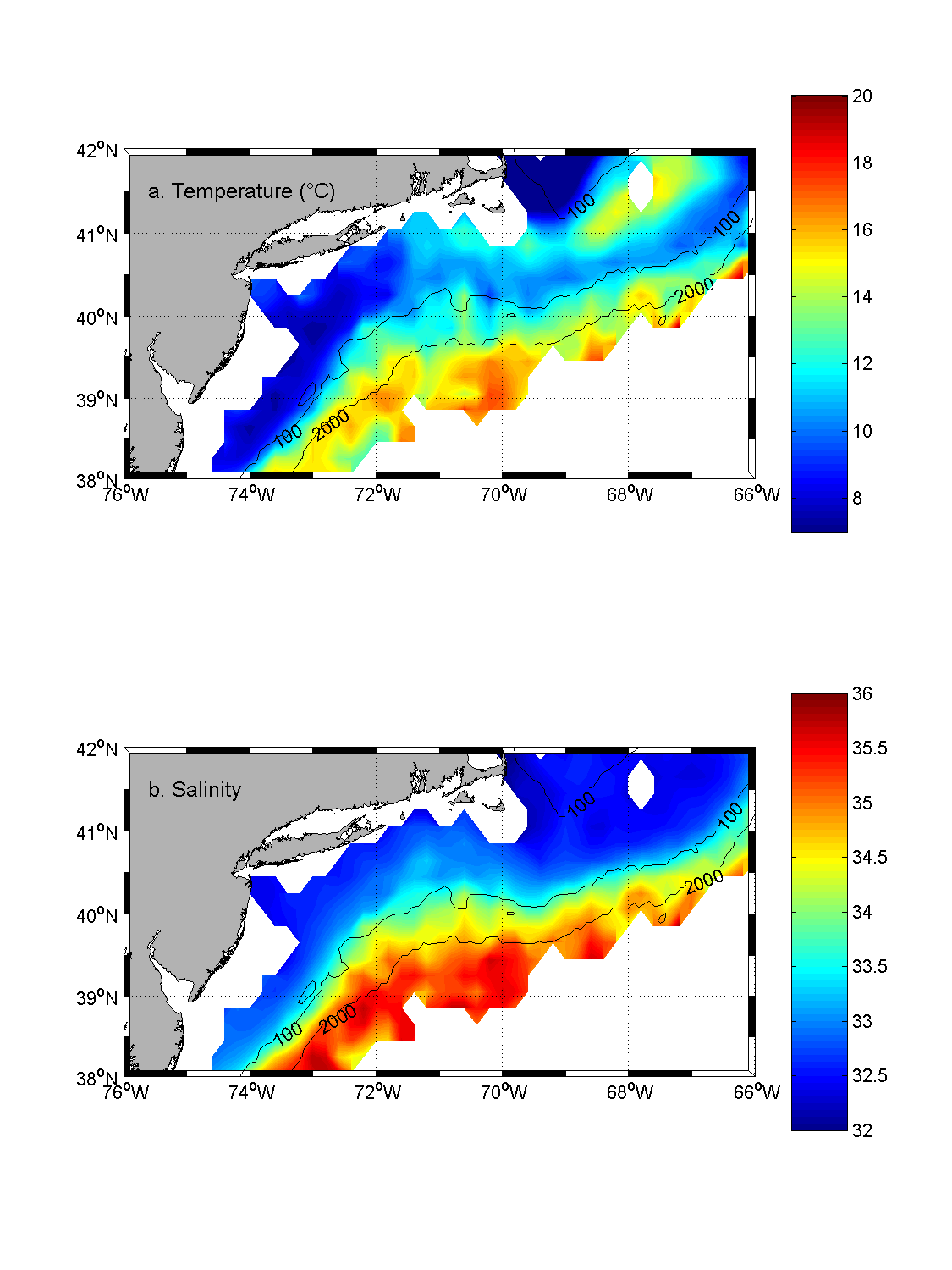
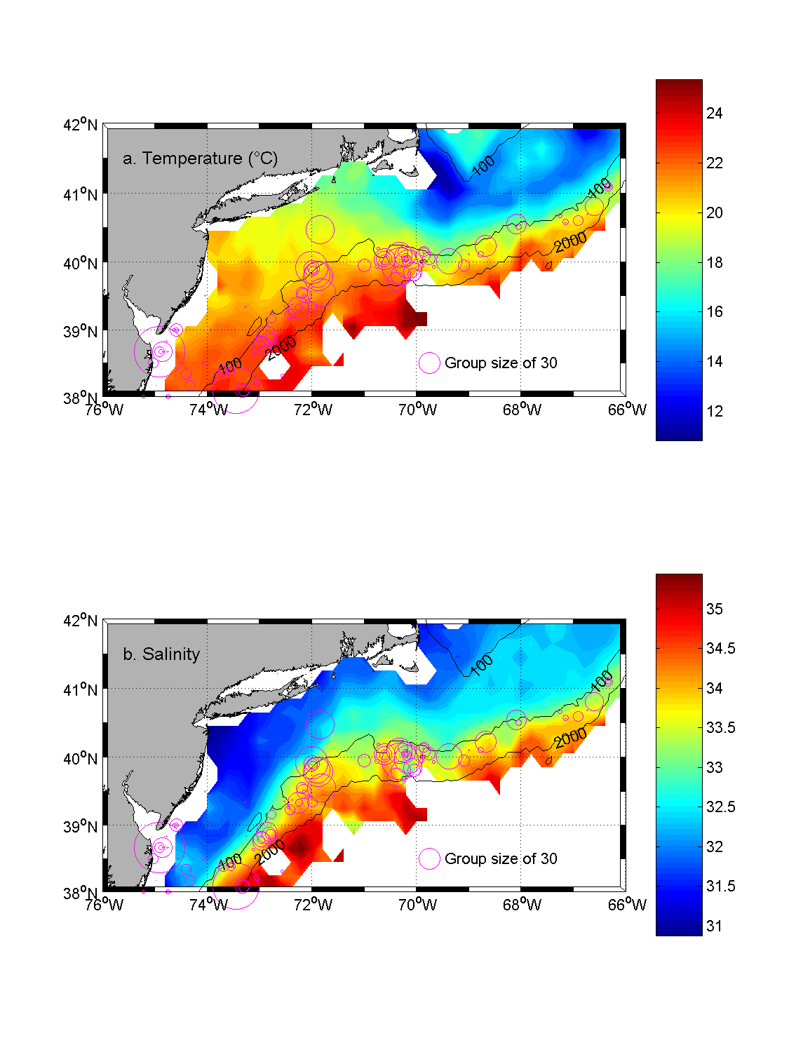
| Figure 1 |
Mean
mid-depth (40-55m) planview climatology (a) temperature and
(b) salinity fields |
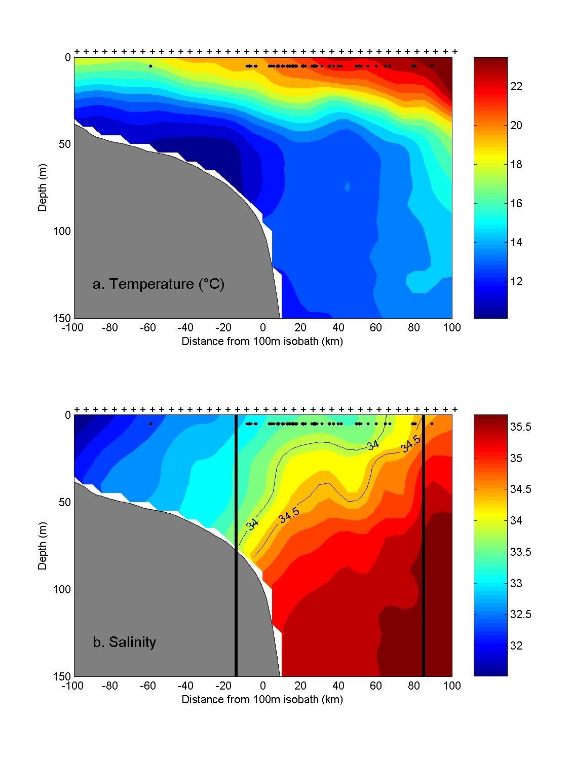
| Figure 2 |
Mean
cross-shelf climatology (a) temperature, (b) salinity, and
(c) density fields. The shelfbreak front is defined by the dark vertical lines at the foot of the front
(intersection of 34.0 isohaline with bottom) and the surface outcrop
(intersection of 34.5 isohaline with surface). |
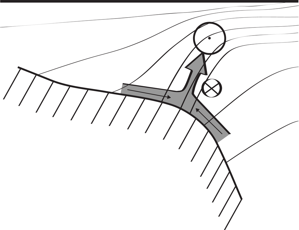
| Figure 3 |
Schematic
of bottom boundary layer detachment in the shelfbreak front |
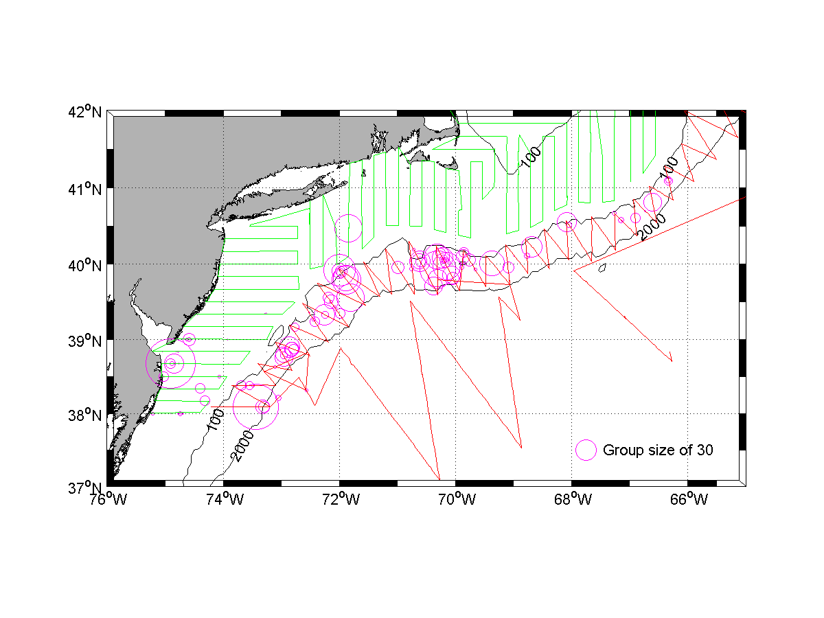
| Figure 4 |
NOAA
summer 1998 marine mammal survey. Green line shows
aerial effort, red line shows ship effort, and magenta circles
indicate sightings (size corresponds to number of individuals
in a group) |
| Figure 5 |
Mean
mid-depth (40-55m) planview climatology (a) temperature and
(b) salinity fields with dolphin sightings overlaid |
| Figure 6 |
Mean
near-surface (5-15m) planview climatology (a) temperature
and (b) salinity fields with dolphin sightings overlaid |
| Figure 7 |
AVHRR images |
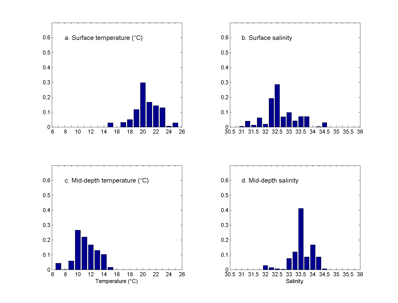
| Figure 8 |
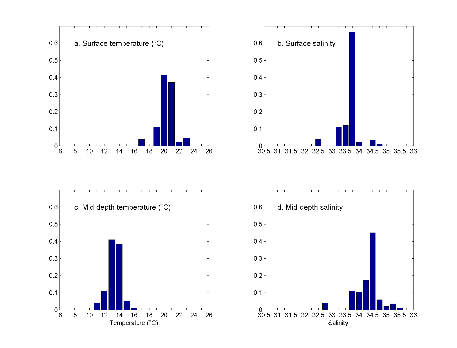
Abundance
of dolphins (normalized by the total number of dolphins) shown
relative to the ABEL-J CTD data (a) surface temperature, (b)
surface salinity, (c) mid-depth temperature, and (d) mid-depth
salinity |
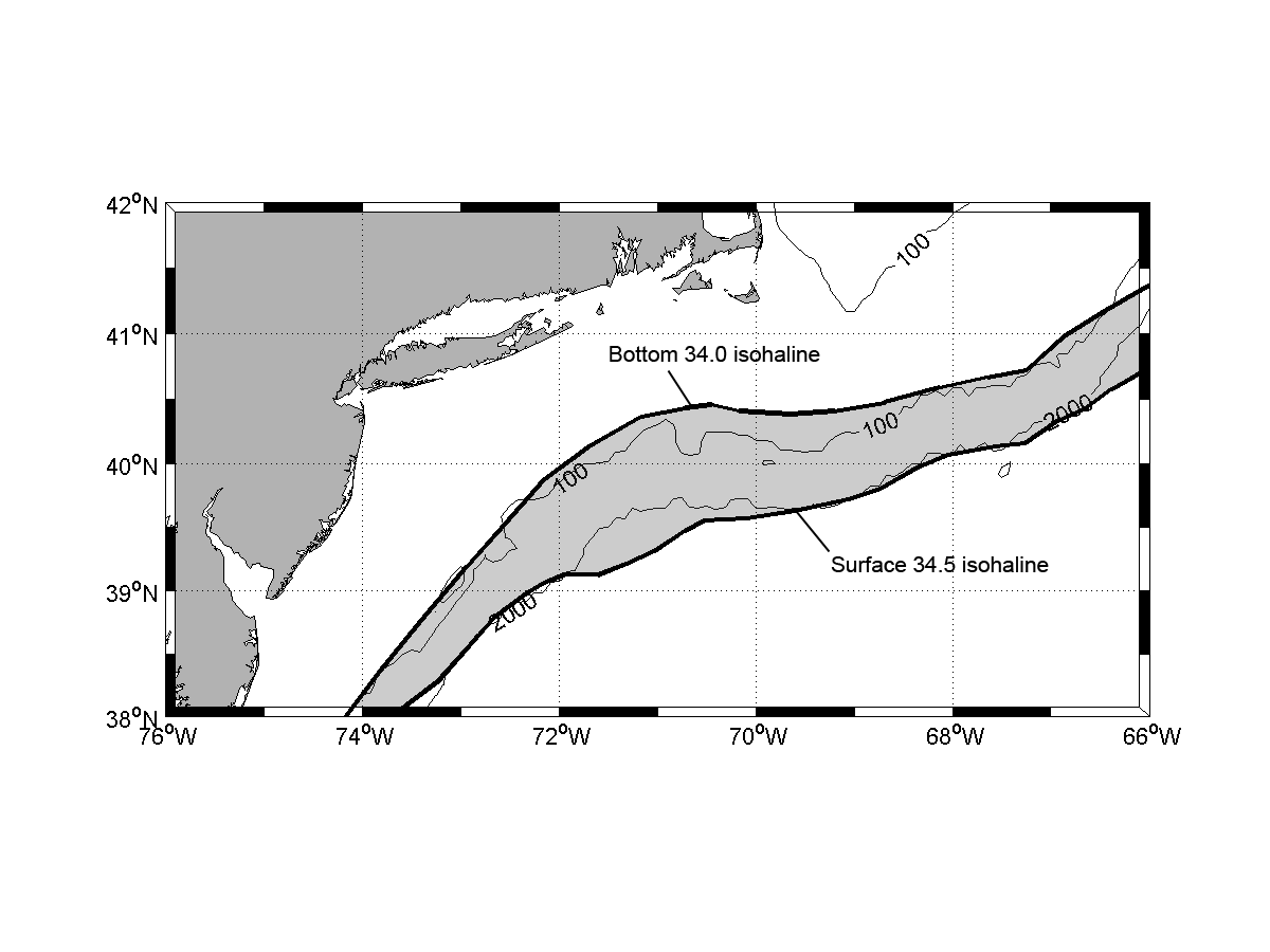
| Figure 9 |
Dolphin
habitat model, defined by the intersection of the 34.0 isohaline
with the bottom and the intersection of the 34.5 isohaline
with the surface. |
| Figure 10 |
Mean
cross-shelf climatology (a) temperature and (b) salinity with
dolphin group sightings overlaid |
| Figure 11 |
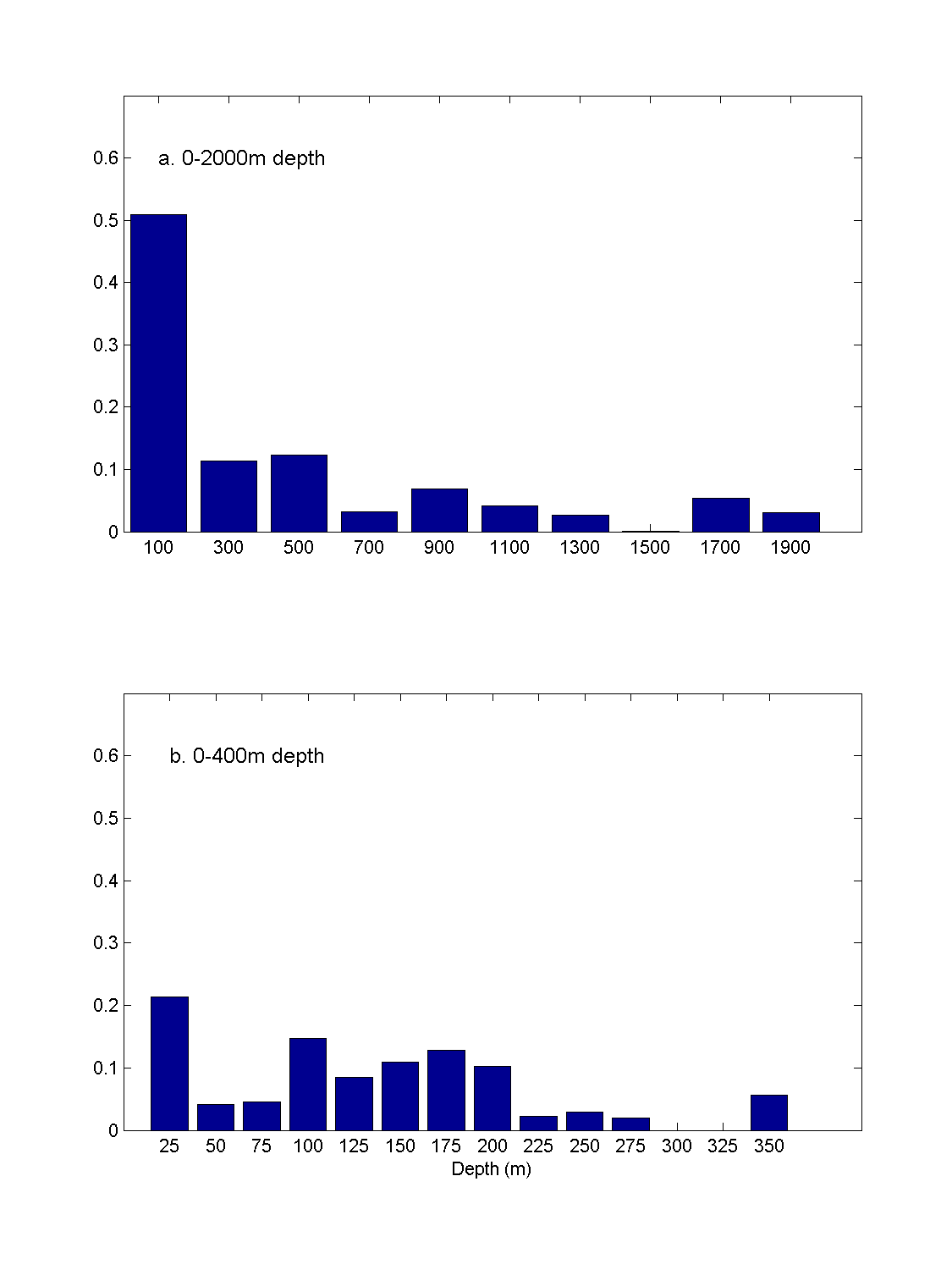
Abundance
of dolphins (normalized by the total number of dolphins) shown
relative to the cross-shelf climatology (a) surface temperature,
(b) surface salinity, (c) mid-depth temperature, and (d) mid-depth
salinity |
| Figure 12 |
Abundance
of dolphins (normalized by the total number of dolphins) shown
relative to the depth (a) 0-2000 meters (b) 0-400 meters |
| Figure 13 |
Random test model results |
This project is funded by the Office
of Naval Research.
|
