
S. T. Bolmer1, R. C. Beardsley1, C. Pudsey2, P. Morris2, P. Wiebe1, E. Hofmann3,
J. Anderson4,
A. Maldonado5
1 Woods Hole Oceanographic Institution
Woods Hole, MA 02543, U.S.A.
2 British Antarctic Survey
Cambridge, CB3 0ET, U.K.
3 Old Dominion University
Norfolk, VA 23529, U.S.A.
4 Rice University
Houston, TX 77251, U.S.A.
5 Universidad de Granada Facultad de Ciencias
18002, Granada, Spain
One objective of the U.S. Southern Ocean Global Ocean Ecosystems Dynamics (SO GLOBEC) program is to gain a better understanding of the sea floor bathymetry in the program study area. Much of Marguerite Bay and the adjacent shelf west of the Antarctic Peninsula were poorly charted when the SO GLOBEC program started in 2000. Before the first SO GLOBEC cruise, an improved local area version (ETOPO8.2A) was created from the Smith and Sandwell (1997) topo_8.2.img 2-minute digital gridded bathymetry for the study area. The first SO GLOBEC mooring cruise on the R/V Lawrence M. Gould (March 2001) showed that the 2-minute spatial resolution of ETOPO8.2A did not resolve many of the canyons and abrupt changes in topography that characterize Marguerite Bay and the inner- to mid-shelf region. It also was not particularly accurate in the more uniform terrain regions. We then decided to collect as much multibeam bathymetry data as possible during the SO GLOBEC broad-scale survey cruises on the R/VIB Nathaniel B. Palmer and combine these data with all other available multibeam and trackline bathymetry data to construct a digital bathymetry database and map for the study area. The resulting database has high-resolution data over much of the shelf and parts of Marguerite Bay gridded at 2 seconds in latitude and 6 seconds in longitude spacing between 65˚ to 71˚ S and 65˚ to 78˚ W. This technical report describes the steps taken to assemble and construct this database and how to access the data via the Internet.
Figure 1. Smith & Sandwell topo_8.2.img data
Figure 3. Comparison of depth data from recent cruise tracks and old navigation charts
Figure 4. GEBCO 2003 1-minute map for SO GLOBEC study area
Figure 5. GEBCO 2003 depth contours
Figure 6. GEBCO 2003 and SO GLOBEC contours
2.4 Other United States Antarctic Program Bathymetry Data
Figure 7. Tracks of SO GLOBEC cruises that collected digital bathymetry data
Figure 8. Tracks of other (non-GLOBEC) USAP cruises that collected bathymetry
Figure 9. USAP R/SV Laurence M. Gould JGOFS Bathymetry used in this compilation
2.5 National Geophysical Data Center
2.8 Lamont-Doherty Antarctic Multibeam Bathymetric Synthesis Database
Figure 10. Tracks of all other cruises in NGDC that collected bathymetry data used in this study
Figure 11. Map of BAS, Spanish, and Russian multibeam bathymetry data contributions
3.1.1 RVIB Nathaniel B. Palmer SeaBeam
3.1.3 British Antarctic Survey Multibeam
3.1.3.1 ASCII XYZ multibeam data
3.2 Conventional echo sounding data
3.2.1 NGDC single point track line
3.2.2 R/V Laurence M. Gould along-track data
Figure 12. All the track coverage with DEM GTOPO30 and SCAR ADD
4 Steps in Getting to a Final Grid
Figure 13. Final SO GLOBEC bathymetric map
Figure 14. Final SO GLOBEC topographic map with elevation coloring
Figure 15. Final SO GLOBEC data, contour interval 100 meters
7 Suggestions for improving the compilation
8 A Brief Time Line of the Compilation
Navigational Charts used to augment ETOPO2-v8.2
Cruises Used to Create the Marguerite Bay Region Bathymetry Chart. 02/01/04
LAND DATA used to Create the Marguerite Bay Region Bathymetry Chart
Programs used in processing the data
APPENDIX 1: MB-System and GMT scripts
Script to grid the Nathaniel Palmer Sea Beam data
Script to grid the Other Multibeam Data
Script to grid the ASCII along track data
Script to merge Land, Gridded at sea data and the SCAR Coastline
Script to find widely divergent points
APPENDIX 2: MatLab Scripts to edit JGOFS data
Figure 16. Main window in JGOFSplot MATLAB GUI tool
Figure 17. JGOFSplot MATLAB GUI tool zoom window
Figure 1. Smith & Sandwell topo_8.2.img data
Figure 3. Comparison of depth data from recent cruise tracks and old navigation charts
Figure 4. GEBCO 2003 1-minute map for SO GLOBEC study area
Figure 5. GEBCO 2003 depth contours
Figure 6. GEBCO 2003 and SO GLOBEC contours
Figure 7. Tracks of SO GLOBEC cruises that collected digital bathymetry data
Figure 8. Tracks of other (non-GLOBEC) USAP cruises that collected bathymetry
Figure 9. USAP R/SV Laurence M. Gould JGOFS Bathymetry used in this compilation
Figure 10. Tracks of all other cruises in NGDC that collected bathymetry data used in this study
Figure 11. Map of BAS, Spanish, and Russian multibeam bathymetry data contributions
Figure 12. All the track coverage with DEM GTOPO30 and SCAR ADD
Figure 13. Final SO GLOBEC bathymetric map
Figure 14. Final SO GLOBEC topographic map with elevation coloring
Figure 15. Final SO GLOBEC data, contour interval 100 meters
Figure 16. Main window in JGOFSplot MATLAB GUI tool
Figure 17. JGOFSplot MATLAB GUI tool zoom window
During the initial planning for the U.S. Southern Ocean (SO) GLOBEC field program, it became very clear that the program would need a better knowledge of the sea floor bathymetry in the program study area if the program was to achieve its’ scientific objectives. Much of Marguerite Bay and the adjacent western Antarctic Peninsula (WAP) shelf were poorly charted, and the coverage of high-quality digital sounding data with GPS-quality navigation data was sparse. Examination of existing maps and along-track data in the U.S. National Geophysical Data Center (NGDC) showed the WAP shelf to be rugged. The area has a mean depth of roughly 500 m but with many canyons and depressions to depths of 800 m interspersed with shallow banks. Marguerite Bay has a more complex bathymetry with George VI Sound having a maximum depth of 1600 m, along with extensive shallows and island groups. Such topographic variability should strongly influence local currents, water properties, and regional circulation, plus biological processes, including animal distributions and behavior (e.g., seal dive depth). Thus, a good knowledge of the bottom topography is essential for both physical and biological sampling and experimental design, data interpretation and physical/biological modeling.
It was evident by the December 2000 SO GLOBEC planning meeting that the program needed to obtain as much new high-quality bathymetry data as possible during the field program if significant improvements to the bathymetry data in the study area were to be achieved. Thus, it was decided to collect high-quality swath bathymetry data during all R/VIB Nathaniel B Palmer (NBP) cruises in the SO GLOBEC study area during 2001-2002. We would merge these data with along-track data collected on the R/V Laurence M. Gould (LMG) and all other multibeam and centerline data that we could obtain. These data would be gridded into a bathymetry database that could be used in planning and scientific analysis by program investigators. Peter Wiebe, Chief Scientist of the NBP 2001 and 2002 austral “fall” and “winter” SO GLOBEC survey cruises, requested that the swath data be collected, and Bob Beardsley agreed to organize and oversee the post-cruise processing and construction of a composite digital bathymetry database for the program.
As a first step towards constructing a better bathymetry we used a digitizing table to determine the latitude and longitude of depth values on existing navigational charts and merged these data with the Smith and Sandwell (1997) topo_8.2.img 2-min digital gridded bathymetry to create the ETOPO8.2A data set. Comparisons with along-track data collected during the March 2001 LMG mooring cruise showed that the 2-min resolution of the ETOPO8.2A data set did not resolve many of the canyons and abrupt changes in topography which characterize Marguerite Bay and the inner- to mid-shelf region, nor was it particularly accurate. At several mooring sites, the pre-deployment site depth survey made with the LMG fathometer bore little resemblance with ETOPO8.2A. This strengthened our desire to collect as much new high-resolution digital bathymetry data as possible in the SO GLOBEC study area during the program field work.
The work of building a composite digital bathymetry database started in earnest in the second half of 2001. High-quality swath bathymetry data were collected on the austral “fall” and “winter” SO GLOBEC broad-scale surveys using the NBP SeaBeam system, and along-track digital bathymetry data from the LMG “fall” and “winter” SO GLOBEC process-oriented cruises. In addition, an extensive multibeam survey was conducted along the deep trough exiting from Marguerite Bay onto the shelf aboard the RRS James Clark Ross in 2001 and made available to us by the British Antarctic Survey (BAS). Center trackline and multibeam data already available at the U.S. Geophysical Data Center (NGDC) also were obtained and incorporated into the map. A first attempt to merge these new data sets with ETOPO8.2A exhibited so much variation with the actual data collected in the study region that we decided to exclude ETOPO8.2A data in future compilations.
Additional multibeam and center trackline data were collected during the 2002 SO GLOBEC “fall” and “winter” NBP broad-scale survey cruises and LMG process-oriented cruises and mooring cruise. Other bathymetric data were from British and Russian sources also were added to the data set. We stopped actively looking for additional data, following the last SO GLOBEC LMG mooring cruise in March 2003, and focused on assembling a final quality-controlled digital bathymetry data set for the SO GLOBEC study region. This new compilation could then be used by interested investigators to produce high-resolution gridded bathymetry maps. This report describes the steps taken to assemble and edit the individual data sets collected in this effort, and the final data set and how to access this data via the Internet. Figure 12 shows the coverage in the area we have assembled from cruise data.
As a first step towards building an improved bathymetry database before any SO GLOBEC cruises in the area, Bob Beardsley and Mike Caruso obtained the Sandwell and Smith topo_8.2.img 2-min digital gridded bathymetry for the SO GLOBEC study area (Figure 1, see http://www.ngdc.noaa.gov/mgg/bathymetry/predicted/explore.HTML for more information about ETOPO2). This bathymetry data set is a merger of satellite-derived data and digital along-track and swath data that had been obtained from the NGDC (see http://www.ngdc.noaa.gov/mgg/geodas/trackline.html ) as of July 15, 2000.
The positions of individual soundings on four published navigational charts (Table 1) in the study area were determined using an XY digitizing table. The resulting digital XYZ data were combined with the above topo_8.2.img data using the GMT program surface. The resulting digital bathymetry data ETOPO8.2A (Figure 2) showed more spatial structure around Adelaide Island and within Marguerite Bay as a result of the addition of the navigational chart data which are not part of the NGDC.
However, as mentioned above, the difference between ETOPO8.2A and depth data collected on the first LMG mooring cruise in March 2001 was so large (Figure 3) that this initial merged product was eventually discarded later that year. We decided not to include the digitized navigational chart data nor the satellite-derived data in ETOPO8.2A in our final data set presented here. The navigational chart data were collected in times when navigation and depth sounding were very crude relative to today’s methods.
Figure 1. Smith & Sandwell topo_8.2.img data. This is a 2-min gridded bathymetry for the SO GLOBEC study area. Note how the shelf break is interpreted in this data set. The Generic Mapping Tools (GMT) coastline is in green. The ADD edge of the ice is shown in blue.
Figure 2. ETOPO8.2A. The increased bumpiness reflects the addition of the navigational chart data before re-gridding. The ADD coastline is in black and ADD edge of the ice is in blue.
Figure 3. Comparison of depth data from recent cruise tracks and old navigation charts. The digitized chart data are plotted as pluses (+) overlying track data. Note the large number of red pluses over areas of yellow and green showing the large differences from the two depth data sets. The black area is deeper than the coloring scheme used. This was left to illustrate the differences in the data sets.
In 2003, the General Bathymetric Chart of the Oceans (GEBCO) published under the auspices of the International Hydrographic Organization (IHO) and the United Nations’ (UNESCO) Intergovernmental Oceanographic Commission (IOC) a 1-min bathymetric data set for the world ocean (see http://www.ngdc.noaa.gov/mgg/gebco/gebco.html). This data set was compiled from a large collection of spot soundings, swath data and satellite-derived data. The compiled data were then plotted and contoured by hand with the resulting contours digitized and gridded to form the final 1-min data set.
The GEBCO interpretation (Figure 4) does not fit well with the multibeam data we have collected in the SO GLOBEC study area. An over-plot of GEBCO contours on a shaded relief map from our data (Figure 5) shows general agreement in some areas and radical differences in others. This is emphasized by the plot of GEBCO contours on our contours (Figure 6), especially over the outer shelf and shelfbreak region. There are also notable differences in coastline and ice shelf edge positions. For this reason, we decided not to use the GEBCO 1-min data. (A discussion group email from Walter Smith about the strengths and weaknesses of the GEBCO 1-min data set can be found at: http://op.gfz-potsdam.de/GMT-Help/Archive/msg09701.html. This note helps explain our omission of the GEBCO bathymetry.)
Figure 4. GEBCO 2003 1-minute map for SO GLOBEC study area.
Figure 5. GEBCO 2003 depth contours. The depth contours plotted in black over the shaded relief plot of the SO GLOBEC data set. The contour interval here is 500 meters.
Figure 6. GEBCO 2003 and SO GLOBEC contours. The GEBCO 2003 and SO GLOBEC contours plotted in blue and red respectively. The ADD coastline is plotted in black and the GEBCO coastline in green. The contour interval here is 500 meters.
SeaBeam swath bathymetry data were collected on the R/VIB Nathaniel B. Palmer (NBP) 2001 “fall” and “winter” and 2002 “fall” broad-scale survey cruises. For the NBP 2002 “winter” cruise there was no operating multibeam system aboard. Thus, only digital centerline echo sounder data were collected and recorded in JGOFS format with the other underway along-track data. The NBP multibeam data were edited at sea during each cruise and are now in good condition. The NBP JGOFS formatted bathymetry data needed extensive post-cruise editing since only limited editing was done at sea. The multibeam data had the sound velocity profiles used in the data processing adjusted at sea. The multibeam soundings data were consistent between each cruise and with the sound velocity profiles agree with data collected from CTD casts taken during the cruise.
On all seven SO GLOBEC R/V Laurence M. Gould (LMG) cruises, digital centerline echo sounder data were recorded in JGOFS format along with other underway along-track data. This JGOFS bathymetry data also needed extensive cleaning as no editing was done at sea. The tracks and swaths where the NBP and LMG collected bathymetry data during the SO GLOBEC field program are shown in Figure 7. The documentation of the sound velocity profile used in collecting the JGOFS data is very poor to non-existant. The good agreement in crossings with the NBP multibeam data showed that this data was useable in our compilation.
Multibeam and centerline bathymetry data collected on other U.S. Antarctic Program (USAP) NBP and LMG cruises in the study area have been obtained for inclusion in our compilation (Figure 8). John Anderson (Rice University) has contributed SeaBeam data from his 1999 NBP geophysics cruise (NBP 99-02) and selected segments of SeaBeam data from his 2002 NBP geophysics cruise (NBP 02-01) in Marguerite Bay. Both of these cruises cover areas that needed coverage and the swath data have been included in the compilation. Centerline data collected on many of the USAP LMG cruises (Figure 9) in the study area from 2000 to early 2003 also have been obtained and included into the compilation (Table 2). As with the other centerline data collected in JGOFS format, the LMG data have required extensive editing to produce accurate depth data (see Appendix 2).
Figure 7. Tracks of SO GLOBEC cruises that collected digital bathymetry data. Also shown in gray are tracks of other cruises that contributed data to the final data set.
Figure 8. Tracks of other (non-GLOBEC) USAP cruises that collected bathymetry.
Figure 9. USAP R/SV Laurence M. Gould JGOFS Bathymetry used in this compilation.
A search of the U.S. National Geophysical Data Center (NGDC) for bathymetric data in our region of interest identified the cruises listed in Table 2 (Figure 10). The majority of these cruises (43 of 46) only had data from 3.5 or 12 kHz centerline recording systems. The bathymetry data have been checked to remove any spurious depths. Since these data were generally not rigorously edited before submission to NGDC and may have been taken with a variety of sound velocities in the water used to calculate depth, a thorough editing and comparison with other data at track crossovers is essential. NGDC has a system of reporting these velocities, but often this seems to be not reported or forgotten when those who collected the data returned from sea.
In addition to the centerline data, we were fortunate to find three multibeam data sets at NGDC. These were of a mixed quality. The data from one Lamont-Doherty Earth Observatory R/V Maurice Ewing cruise has the overall crude bathymetry in the right range but the actual data points need further editing. These data are in areas that fills gaps in our coverage but this cruise data must be used with care. Two multi-beam cruises attributed to NOAA seem to have data that fits in well and looks fairly cleanly edited.
We were fortunate to make contact with Carol Pudsey and Peter Morris at the British Antarctic Survey (BAS) near the beginning of the SO GLOBEC field program. They have provided us with extensive multibeam data from their 2001 and 2002 RRS James Clark Ross (JCR) geophysics cruises in Marguerite Bay (Figure 11). These cruises mapped large parts of Marguerite Trough, the channel that leads from to the shelf break from the mouth of Marguerite Bay and George VI Sound. Since the Marguerite Trough is such a dominant topographic feature in the region, the high-quality multibeam data from these BAS surveys have been crucial additions to our data set.
During the summer of 2003, Carol and Peter provided us with raw multibeam data from several other JCR cruises in the SO GLOBEC study area. These data had not been edited beforehand and after editing by Tom Bolmer have been added to our data set. These surveys have added many new and useful miles of new data to this study. In the winter of 2004 Rob Lartner sent us trackline date from the JCR that go along the shelf and the rise.
Peter also provided edited multibeam data collected on a 1991 geophysics cruise abroad the Russian ship R/V Academik Boris Petrov. This cruise included several tracks along the shelf that parallel themselves and cross the SO GLOBEC tracks at right angles, thus providing very useful tie lines. Some of the Russian data were discarded in the deeper water areas off the shelf, where they did not agree with our other data there. The data on the shelf areas is not without its' problems. But, since these data cover areas that need coverage it has been left in. We have done some further editing of these data in shallower areas. The editing has been cumbersome since the data are only in an ASCII XYZ format and thus it is hard to remove points from easily.
Rob Larter at the BAS provided MGD77 formatted data for 2 tracks from the JCR cruise JR04 in 1993 that follow the shelf break on the shelf and out on the continental rise (Figure 11).
Andrés Maldonado (Instituto Andaluz de Ciencias de la Tierra, Universidad de Granada, Spain) contributed the gridded multibeam bathymetry data set from the ANTPAC97-98 geophysics cruise on the R/V Bio-Hesperides. This data set improved the density of coverage at the shelf break in one area (Figure 11).
The Lamont-Doherty Earth Observatory Antarctic Multibeam Bathymetric Synthesis Database web site ( http://data.ldeo.columbia.edu/antarctic/ ) provided us with several USAP data sets that were not available elsewhere. These cruises have helped fill in some areas in the north east regions that had few cruises. As of this date this site has two large multibeam data sets that have not been released. We are using the underway JGOFS bathymetry for both of these, but we do have a partial set of the multibeam data released to us for one of the cruises. These two cruises should be available in early 2004 after the 2 years proprietary time for these data is up. At the time of this report one of the chief scientists for these cruises has put an additional 6 month hold on releasing the data from his cruise.
Laurie Padman (Earth and Space Research, Seattle) contributed the bathymetry data used in his tidal models for the study region. In particular, his data set has a 1/4 degree longitude by 1/12 degree latitude grid with coverage under the Wilkins Ice Sheet and George VI Sound. While this is very coarse spacing, it does help constrain the land and other bathymetry in our study area. Laurie based his data base on an Oregon State University global tidal solution based on the ETOPO-5 data. The web-site describing this data is at: http://www.ers.org/antarctic/barotropic.html#CAT .
From Maslanyj (1987) we used 3 profiles across George IV Sound. These data were collected using seismic techniques. There are only three profiles that we can use in the area but they show us that George IV Fjord is a channel around Alexander Island. These profiles can be seen in Figure 12.
Figure 10. Tracks of all other cruises in NGDC that collected bathymetry data used in this study.
Figure 11. Map of BAS, Spanish, and Russian multibeam bathymetry data contributions. The red and pink like BAS data and the blue Spanish data were sent as ASCII XYZ data and those points are plotted here instead of a cruise track.
We have relied on publicly available programs to create the final bathymetry data set presented here. In particular, we have used the MB-System software written by David Caress (Monterey Bay Aquarium Research Institute) and Dale Chayes (Lamont-Doherty Earth Observatory). This software package was developed with NSF support and is described at http://www.ldeo.columbia.edu/MB-System/MB-System.intro.html . This software allows editing and converting the multibeam data into latitude-longitude gridded data that we can then manipulate and merge with other data.
We also have used the Generic Mapping Tools (GMT) written by Paul Wessel (School of Ocean and Earth Science and Technology, University of Hawaii) and Walter Smith (NOAA Laboratory for Satellite Altimetry) (see http://gmt.soest.hawaii.edu ). These programs were used to merge and do the rest of the gridding and plotting of the data. See Appendix I for examples of the scripts we had not previously noticed.
In the process of sorting, editing, and managing the various data sets, we have also developed PERL and MatLab programs as needed. We also have used the sh and csh shells, the generic shell scripting inherent in UNIX, to manage the data and run the processing steps we used. All final processing was done on a Sun Ultra 60 UNIX workstation running Solaris 8.0 with nearly 150 GB hard disk drive storage. Brief descriptions of the processing done on various data sets are presented next.
We were fortunate to recently have the Interactive Visualization Software company's Fledermaus program available to us. This program was able to read in the gridded NETCDF data from GMT and plot the data in Three Dimensions (3D). By being able to rotate and fly through the 3D figure we were able to find large highs and lows that were previously missed. We then went back to the raw data and removed the extraneous points and ran through the whole process to make a gridded data set again. By using this 3D and editing process several times were able to remove the abnormalities. There are some examples of the Fledermaus figures on the data web site referred to below.
Multibeam systems considered here provide up to 150 and more depth points on a swath (transect) perpendicular to the ship’s track. The width of the swath is typically 1.5 times the water depth, so this swath measurement approach is much more effective in mapping areas than the along-track single-point echo sounder. The raw multibeam data requires careful visual editing of individual ping data, a major labor-intensive effort. We have used the MB-System mbedit program for editing raw multibeam as needed, and the MB-System mbgrid program to convert the edited multibeam swath data into equally-spaced latitude, longitude, depth (xyz) values.
The multibeam data collected on the R/VIB Nathaniel B. Palmer were edited by the scientific party on board the ship at the time of collection. The efforts of the scientific party were coordinated and quality controlled by the Raytheon Polar Services shipboard technicians. In addition to overseeing the basic swath editing, the technicians also checked the navigation data input and made corrections as needed. This thankless job was done on all cruises and has made this digital data base construction possible.
NGDC had three multibeam data sets collected in the study area. At this time, we have used these data without editing, although we recommend further editing of these data sets.
The British Antarctic Survey has supplied both edited processed and raw multibeam data. The processed data were in ASCII xyz format. These data sets have been used without change. They do exhibit some spatial distortion due to the space scale used in the gridding. If possible, we will attempt to obtain the original edited multibeam files to include in the final database.
The BAS raw multibeam data had been collected with a Simrad 120 multibeam system that used a data storage format that could not be edited directly by MB-System. The raw data were first converted into a format compatible with MB-System, then edited with mbedit. A few sections needed sound speed adjustment. These data are now edited and included in the current version of the SO GLOBEC data base.
A large part of the digital bathymetry data in the study area was collected using more traditional echo sounders. This type of data provided the largest number of miles of data along track. This type of echo sounding only provides a single depth point under the ship, unlike the swath data from the multibeam mapping systems.
These data need quality control checking. The data were provided to NGDC from many sources, and while many sources provide processed data, some only provide raw (unprocessed and unchecked) data. There are no real quality control tags on the data provided to NGDC, so care must be made to check the crossings of the along-track data between individual cruises. Sometimes the data will show differences of 10’s (to even 100’s) m between the depths from two cruises at a crossing point. This difference must be resolved before utilizing the data from either cruise.
Although these along-track data cover a small area of the map relative to that area covered by the multibeam data, the along-track data are critical in providing coverage of the region and “tie lines” to the multibeam data. These tie lines can be used to constrain valleys and ridges and help confirm regional trends.
The NGDC along-track data were processed using the MB-System program mbgrid to create a gridded data set to use with data from other sources.
We have been fortunate to get access to the along-track single-point bathymetry data collected during 2000-2003 on the R/V Laurence M. Gould (Figure 9). The ship’s data acquisition system records 1-min data from a suite of underway meteorological and water sampling systems that include the ship’s digital echo sounder and GPS latitude and longitude. The data are stored in the Global Ocean Flux Study (JGOFS) ASCII format. The echo sounder uses its own bottom detection software and the data must be carefully edited to remove the many spurious depth values that occur, especially when the ship is working in the ice. Tom Bolmer wrote a MatLab program (see Appendix II) to identify and remove spurious data plus obvious peaks and valleys in the data that are unreasonable relative to what is known about the area or relative to other data (Figures 16 and 17).
The resulting edited JGOFS depth and position data were then processed with the MB-System program mbgrid to create a gridded data set that can be merged with data from other sources.
Peter Morris provided the Scientific Committee on Antarctic Research (SCAR) 1:1 million Antarctic coastline data set (http://www.nerc-bas.ac.uk/public/magic/add_home.html). This is the current version of the coastline for the region. The GMT coastline subroutine in the GMT suite of programs uses data from old navigation charts of the area so that the GMT coastline is only useful for gross features. During cruises in the area, ships have “sailed” past the GMT/navigational chart coastlines onto “land”. We have used the SCAR coastline data to constrain the areas with very little data and define the coastline in our gridded data (figure 12).
We have downloaded the United States Geological Survey global Digital Elevation Model (DEM) (GTOPO30) (http://edcdaac.usgs.gov/gtopo30/gtopo30.html) to use for the land area (Figure 13). This data set has a horizontal grid spacing of 30 arc seconds (approximately 1 kilometer), and covers most of the region except for some of the smaller islands in the northeast and southwest which are likely too small to be resolved with the 30-sec grid spacing. The DEM data have helped constrain the bathymetry by having the topography to influence the gridding of the bathymetry.
Figure 12. All the track coverage with DEM GTOPO30 and SCAR ADD data. The DEM data is shown on land. The SCAR coastline and ice edges are shown. There is good agreement between the two data sets within the 30-sec spacing of the GTOPO30 data.
All of the data sources and types mentioned above were used to create a final data set and bathymetric chart. We first created a series of grids from some of the different data types and then merged them together with some sources getting preference. The steps we followed to create the final products are listed below. The scripts used to create these files are included in Appendix 1. Table 4 has a list of the programs used in the processing. The final version of the data set can be seen in Figures 13, 14 and 15.
9. All of the ASCII XYZ data files were concatenated together into a single file. These files are: a) the ASCII XYZ ship bathymetry data, b) the ASCII XYZ GTOPO30 land elevation data, c) the ASCII XYZ SCAR ADD coastline data, d) the ASCII XYZ file of bathymetric soundings in the King George VI Sound, and e) the ASCII XYZ data sent by Laurie Padman for use in areas of ice sheets.
10. This single XYZ file was then searched using the UNIX program egrep to remove those locations where there was no data. The NaN values were removed in this step, leaving only XYZ points with real data.
11. The GMT program blockmedian was then run to get a median position and value for every non-empty block in a grid “cell”. Grid locations with data in them were created, thus generating a grid with either data or no data in equally spaced locations from the irregularly spaced input data.
12. The resultant file from the program blockmedian was then processed with the GMT program surface. Surface smoothly fills in empty grid locations with an interpolation sheet passing through the existing grid cells with data. The resulting grid can then be used to create maps of the study area. We used a grid spacing of 6 seconds longitude and 2 seconds of latitude. The program surface could not use meters as a grid spacing. These grid spacing values in surface best fit those output from the mbgrid program.
13. The grid above was input into the IVS Fledermaus program to find largely divergent highs and lows in the data set. The raw data were plotted in these regions to help find and remove the bad data points from the data set.
14. The data center line data were then regridded, and merged with the multibeam data again. Then steps 10 to 12 from above were repeated. The process of doing steps 13 and then redoing 10 to 12 was done several times until no more large diversions were noted in the data set with Fledermaus.
Figure 13. Final SO GLOBEC bathymetric map.
Figure 14. Final SO GLOBEC topographic map with elevation coloring.
 >
>
Figure 15. Final SO GLOBEC data, contour interval 100 meters.
To facilitate the initial distribution of this data set to the SO GLOBEC participants, the web site http://www.whoi.edu/science/PO/so_globec/ was created to allow participants to download the data set. This web site has a link to an ftp site. The ftp site has a user name and password associated with it. For the time period that the data are proprietary. Since the SO GLOBEC participants use such a large range of computer operating systems and software, it was hard to find a single kind of data format that would be useful to all. As a result, we decided to serve on the ftp site the data set in the following formats:
1. GMT-created NetCDF binary files with 3 grid resolutions to allow users with smaller computers to get the data and be able to work with the files. These were a 6seconds longitude and 2 seconds latitude grid, a 15 seconds on each side grid and a 1 minute on each side grid.
2. ASCII XYZ files with 2 grid resolutions for the same reason. Only the 15 seconds and 1 minute grids were used here due to file size limitations.
3. Separate ASCII XY files for each 100-m depth contour.
4. MatLab MAT files of the gridded data with two different grid resolutions. We used the same size grids as in number 2 above.
5. A TIFF file for GIS users. (We have had trouble distributing data to users of GIS software packages. These programs seem unable to read the NetCDF-formatted files nor re-grid the ASCII XYZ data easily. This TIFF file is an attempt to get the GIS users data they can use.)
6. GIS users have a separate directory of files provided by Ari Friedlaender (Duke University). (The format of these files is not understood by us.) Other GIS users have had trouble using these files also. These files are still being served in the hope that they are helpful to someone.) At the time of publication these GIS files are not of the current gridded data set. We hope to have that updated soon with help from other SO GLOBEC participants.
7. There are two scene files for use in the IVS iView3D program. These files used with the free program iView3D program will enable the user to "fly" though the data in a 3D grid.
With the publication of this technical report, the web site http://www.whoi.edu/science/PO/so_globec/ will be updated and the digital bathymetry ftp site ftp.whoi.edu , which has the username of so_globec, will be opened for all users. Another link to these sites will be added to the U.S. Southern Ocean GLOBEC website at Old Dominion University ( http://www.odu.edu/Research/globec_menu.html ) to help dissemination of the existence and availability of this data set. The GLOBEC web site at W.H.O.I. for the distribution of all U.S. GLOBEC data (Georges Bank, NEP, and SO GLOBEC) also has a link to this data at: http://globec.whoi.edu/jg/dir/globec/soglobec/ . The complete SO GLOBEC digital bathymetry data set will be archived at WHOI by Tom Bolmer (tbolmer@whoi.edu) and investigators seeking data products not present on the ftp site should contact Tom directly.
By combining bathymetric data from many sources and using various interpolation methods, a data set of bathymetry gridded nominally at 75-m spacing and bounded by 65o to 71o S and 65o to 78o W has been created. This represents a significant improvement over what was previously available in this area. The final product in the form of several gridded depth and depth contour data sets using different horizontal resolutions will now be available to all users (both the SO GLOBEC investigators and the rest of the public) at the ftp site: ftp.whoi.edu ( ftp://so_globec@ftp.whoi.edu ) , at the web site: http://www.whoi.edu/science/PO/so_globec/ , and at the US GLOBEC web site at: http://globec.whoi.edu/jg/dir/globec/soglobec/ .
This compilation is only a snap shot of the data available at the time of publication of this report. There are many things that could be done to improve upon this bathymetry data set. We listsome ideas below.
1) We are confident that we have found most of the science cruises in region that collected well-located digital bathymetric data. But we feel that we have not gotten all of those available.
2) Some of the data that we have could be improved upon by having access to the processed multibeam files instead of more coarsely gridded ASCII XYZ data.
3) There are several cruises included in this compilation for which only a limited subset of the bathymetry data was made available to us. Including the missing data from these cruises would improve the accuracy in some areas.
4) In the process of editing the single channel track data, we may have erred and edited out good data points. It is very difficult to edit and process this type of data without access to the actual echo sounding records for comparison. Several examples of undiscovered shoals were found in the echo sounding data on the SO GLOBEC RVIB N. B. Palmer cruises that were not shown in the edited single channel track data. These omissions should be investigated further.
5) Some of the data could benefit from further processing. We perhaps would be able to improve upon the map we have if we could process the entire data set with the new bathymetry processing tool now in development and testing at the University of New Hampshire.
6) The final gridded product could be improved by having a surfacing routine that smoothes the areas with no data in a better more realistic manner. The currently used GMT program is not producing smoothly flowing surfaces.
7) There should be some way to incorporate larger data sets like the Smith & Sandwell 2-minute gravity-derived topography, the GEBCO 2003 1 minute grid or the SCAR BEDMAP data set into this SO GLOBEC compilation.
At this moment, there is a large difference between our product and these. Since we have a larger data set in a smaller area than these compilations, our data should be able to guide these data sets in our region of interest. If we could use our data set (which is more complete and accurate in our study region) as a ground truth data set for one of these products, perhaps we could utilize the resulting other product to make a more complete bathymetry map for our region.
8) There are regions in the map area where additional data could make a large improvement. These areas can be seen easily by looking at Figure 12. There are large areas where there is very sparse data coverage. Several of the areas we think that need more survey work done are:
a) The region off of Lazareth Bay. It would be good to see if the deep area near the bay continues offshore. Does this deep continue further onshore?
b) Both the Wilkins and George VI Ice Shelves need more data. Only Maslanyj's profiles in George VI Sound contain any real data in these areas.
These areas probably contribute to the general circulation in the region with water passing under the ice shelves. Knowing how much water could possible move in these regions would help modelers in the general region.
c) The general southwestern part of the map needs more data collected. There are hints of features but the existing data are so sparse that we need more data to constrain these features. Does the deep in the southwestern area continue over the continental shelf to the deep sea?
d) There has been scientific interest in a more-detailed description of the bathymetry in the Crystal Sound area. There are questions as to whether the deeper areas are connected to the shelf. Deeper water mass characteristics have been noted in the area and it would be good to know if there is a channel for this water to get there.
e) The southeastern part of Marguerite Bay to the east of Marguerite Trough shows no cruise tracks in the area. The general interior of Marguerite Bay is only sparsely surveyed. Having a better idea of the bathymetry here would help a lot in understanding the overall Marguerite Bay system.
Get Smith & Sandwell 2 minute global elevation data
check and get NGDC track lines data
digitize Navigational charts
Merge all of this into a new ETOPO82A gridded data set
First R/V Laurence M. Gould SO GLOBEC Cruise LMG0102 Data are noted to be VERY different from the ETOPO82A data
Begin first of three RVIB Nathaniel B. Palmer SO GLOBEC cruises collecting SeaBeam data. Data are processed at sea.
After the first two cruises we tried to merge all of the data assembled to date.
These data are noted to not merge very well with the ETOPO8.2, the ETOPO82A or the digitized Navigation charts.
A decision is made to not use any of the previously assembled data. We will only collect our own data and search for other available data sets.
Carol Pudsey at British Antarctic Survey offers the data from a multibeam cruise on the James Clark Ross.
Do a search of NGDC and get all bathymetry data available. This includes a few cruises that collected multibeam. Get the GTOPO30 30 second spaced topography data. This fills in the land areas and helps constrain the data set.
Peter Morris sends the SCAR ADD coastline data. We tried to get this from the ADD web site but it is only distributed in GIS files. Could not read the GIS data formats so the ASCII files from Peter are a great help. This constrains the bathymetry data set to the water area only when we are using surface to fill in unsurveyed areas.
Created a tool to edit out bad data points from the R/VLaurence M. Gould and RVIB Nathaniel B. Palmer underweigh “JGOFS” meteorology data. These data included bathymetry from the either the 3.5 or 12 kHz echo sounders. These data were NOT edited for quality control at sea. This MatLab tool helped by being able to remove extraneous points, using the GUI tools in MatLab. Wildly different peaks and valleys were removed this way.
Peter Morris at the BAS puts me in touch with Andras Maldonado in Spain who offers multibeam from the Hesperides.
Presented a poster at the Ocean Sciences AGU Hawaii February 2002 to show the process of the work.
After SO GLOBEC cruise III on the RVIB Nathaniel B. Palmer some data wre also released by previous chief scientists on the RVIB Nathaniel B. Palmer . SO GLOBEC cruise III is the last SO GLOBEC to collect multibeam data. The SeaBeam system on the RVIB Nathaniel B. Palmer was replaced by a Simrad system, which was not operational at cruise time for SO GLOBEC IV.
Created a web site to show the AGU poster on line. This was added to as new things were done to the data. Before the 2002 December SO GLOBEC meeting the first set of preliminary data was put up on the web for SO GLOBEC participants to down load and use.
BAS sent raw multibeam data from cruises in the area. These were data that had not been processed due to lack of interest at BAS. Tom mbeditted the data in the summer of 2003 and added it to the collected data.
Searched through the data and added points to areas where no data existed. Data from Laurie Padman were used to fill in areas like under the Wilken's Ice Shelf where we had no data. We needed to edit Laurie's data so that is did not occur on land or in areas we had real ship track data. We also added points to areas that Laurie's data did not cover but where we had coastline and land elevation data. This helped constrain some areas to give surfaces that fit the general data available. This was basically an adjustment to the data to force the computer surfacing and gridding programs towards more realistic results.
Acquire the GEBCO 2003 world 1 minute gridded data set. This turns out to be of no use. The grid was made by digitizing hand contoured data and then re-gridding the data. The data utilized were not as current a data set as we have. This produced a product that is very different from the real data we have assembled. It had been hoped that the data set could be a back drop to the data we have collected.
IVS Fledermaus program available to 3D viewing. This was used to highlight regions with previously unnoticed spurious highs and lows. These points were then removed and the data regridded in mbgrid. The rest of the data flow was then repeated to get a final gridded product.
Rob Lartner at BAS sent 2 single channel tracks of bathymetry data from the RRS James Clark Ross as the final parts of this report were being checked prior to publication.
We want to thank the many individuals who have helped collect and edit the multibeam and along-track bathymetry data included in this SO GLOBEC digital bathymetry data set. Without their effort, both at sea and back home, this project could not have happened. The resulting data set and our improved knowledge of the bathymetry in Marguerite Bay and adjacent shelf is a direct result of many individual decisions to collect high-quality data and share these data with others.
We also wish to thank Walter Smith for the helpful advice and comments he provided during this project.
This work has been supported by the U.S. National Science Foundation through grants OPP 99-10092 and OPP 02-34163 to Bob Beardsley and Tom Bolmer (WHOI), OPP 99-10307 to Peter Wiebe (WHOI), OPP 99-09956 to Eileen Hoffman (ODU), OPP 95-278776 to John Anderson (Rice), and the British Antarctic Survey (Natural Environment Research Council). This support from NSF and BAS is greatly appreciated.
Caress, D. W., and D. N. Chayes, New software for processing sidescan data from sidescan-capable multibeam sonars, Proceedings of the IEEE Oceans 95 Conference, 997-1000, 1995.
Caress, D. W., and D. N. Chayes, Improved processing of Hydrosweep DS multibeam data on the R/V Maurice Ewing, Mar. Geophys. Res., 18, 631-650, 1996.
GTOPO30, Global Topographic Data. Land Process Distributed Active Archive Center (LP DAAC), U. S. Geological Survey's EROS Data Center, http://edcdaac.usgs.gov (http://edcdaac.usgs.gov/gtopo30/gtopo30.html).
IOC, IHO, and BODC (2003). Centenary Edition of the GEBCO Digital Atlas. Published on CD-ROM on behalf of the Intergovernmental Oceanographic Commission and the International Hydrographic Organization as part of the General Bathymetric Chart of the Oceans; British Oceanographic Data Centre, Liverpool.
Maslanyj, M. P. (1987). Seismic bedrock depth measurements and the origin of George VI Sound, Antarctic Peninsula. British Antarctic Survey Bulletin, 75, 51-65.
SCAR Working Group on Geodesy and Geographic Information, Antarctic Digital Database ,Version 3.0, http://www.nerc-bas.ac.uk/public/magic/add_main.html, July 2000, Scientific Committee on Antarctic Research.
Smith, W. H. F., and D.T. Sandwell (1997). Global Sea Floor Topography from Satellite Altimetry and Ship Depth Soundings. Science, 277, 1956-1962. http://topex.ucsd.edu/WWW_html/mar_topo.html
Wessel, P., and Smith, W. H. (1991). Free Software helps Display and Map Data. EOS Trans., 72, 441,445-446.
Wessel, P., and Smith W. H. (1998). New, improved version of the Generic Mapping Tools released. EOS Trans., 79, 579.
| Map | Description |
GB 3571 |
Lavoisier Island to Alexander Island U.K. Hydrographic Office (fm) 1:500 000 10/1/1998 |
GB 3577 |
Adelaide Island, South Western Approaches U.K. Hydrographic Office (fm) 1:75 000 3/1995 |
US 29142 |
Alexander Island to Square Bay, including Marguerite Bay National Imagery and Mapping Agency (m) 1:200 000 11/2/1996 |
US 29141 |
Square Bay to Matha Strait, including Adelaide Island Defense Mapping Agency (m) 1:200 000 8/6/1988 |
Cruise |
Center Beam |
Multi-Beam |
NSF NBP0103 |
X |
|
NSF NBP0104 |
X |
|
NSF NBP0201 |
JGOFS (the rest) |
X (selected) |
NSF NBP0202 |
X |
|
NSF NBP0204 |
JGOFS |
|
B.A.S. JR59 |
X (XYZ file) |
|
B.A.S. JR69 |
X (XYZ file) |
|
B.A.S. JR71 |
X (XYZ file) |
|
LDEO EW9101 |
X |
|
NOAA RITS93A |
X |
|
NOAA RITS94B |
X |
|
RUSSIA Petrov 1991 |
X (XYZ file) |
|
SPAIN Hesperides ANTPAC97-98 |
X (XYZ file) |
|
NSF LMG0009 |
JGOFS |
|
NSF LMG0101 |
JGOFS |
|
NSF LMG0102 |
JGOFS |
|
NSF LMG0103 |
JGOFS |
|
NSF LMG0104 |
JGOFS |
|
NSF LMG0105 |
JGOFS |
|
NSF LMG0106 |
JGOFS (Discarded) |
|
NSF LMG0201 |
JGOFS |
|
NSF LMG0201A |
JGOFS |
|
NSF LMG0202 |
JGOFS |
|
NSF LMG0203 |
JGOFS |
|
NSF LMG0205 |
JGOFS |
|
NSF LMG0301 |
JGOFS |
|
NSF LMG0302 |
JGOFS |
|
LDEO C1503 |
MGD77 |
|
LDEO ELT10 |
MGD77 |
|
LDEO ELT43 |
MGD77 |
|
LDEO THA80 |
MGD77 |
|
LDEO THB80 |
MGD77 |
|
W.H.O.I. PD388L01 |
MGD77 |
|
W.H.O.I. PD190L02 |
MGD77 |
|
RICE UNIV. DF85 |
MGD77 |
|
RICE UNIV. DF86 |
MGD77 |
|
RUSSIA Ioffe 1992 |
MGD77 |
|
S.I.O. DSDP35GC |
MGD77 |
|
U K RRS Bransfield 1985 |
MGD77 |
|
U K HMS Endurance 1985 |
MGD77 |
|
U K RRS Discovery 1887 |
MGD77 |
|
U K HMS Endurance 1987 |
MGD77 |
|
U K HMS Endurance 1988 |
MGD77 |
|
U K RRS Charles Darwin 1989 |
MGD77 |
|
U K HMS Endurance 1991 |
MGD77 |
|
U K HMS Endurance 1992 |
MGD77 |
|
U K HMS Polar Circle 1992 (139) |
MGD77 |
|
U K HMS Polar Circle 1992 (144) |
MGD77 |
|
U K HMS Endurance 1994 |
MGD77 |
|
U K HMS Endurance 1996 |
MGD77 |
|
U K HMS Endurance 1997 |
MGD77 |
|
U K HMS Endurance 1999 |
MGD77 |
|
U K RRS James Clark Ross JCR10L01 |
MGD77 |
|
U K RRS James Clark Ross JCR10L02 |
MGD77 |
|
U K RRS James Clark Ross JCR04 |
MGD77 |
|
BRAZIL TF88-89 |
MGD77 |
|
ARGENTINA IRI93-94 |
MGD77 |
|
ARGENTINA AI9495 |
MGD77 |
|
ARGENTINA BHPD9798 |
MGD77 |
|
NSF NBP92-8 |
MGD77 |
|
NSF NBP93-7 |
MGD77 |
|
NSF NBP93-8 |
MGD77 |
|
NSF NBP94-2 |
MGD77 |
|
NSF NBP95-7 |
MGD77 |
|
NSF NBP99-2 |
X |
|
NSF NBP99-3 |
X |
|
NSF NBP99-5 |
X |
|
NSF NBP99-6 |
MGD77 |
|
NSF NBP00-1 |
MGD77 |
|
NSF NBP00-4 |
MGD77 |
|
NSF NBP01-5 |
MGD77 |
|
NSF NBP01-7 |
MGD77 |
|
UNIV TOKYO UM66-B |
MGD77 |
|
ODP LEG 178JR |
MGD77 |
Data is in the form of XYZ and in the best spacing available. |
GTOPO30 |
SCAR ADD coastline data |
GEORGE VI Sound Soundings traverses (Maslanjy) |
MB-System |
Caress, Spitzak, and Chayes |
|
GMT |
(Generic Mapping Tools) |
Wessel and Smith |
PERL |
(Practical Extraction and Report Language) |
Wall |
MatLab |
MathWorks |
|
Fledermaus |
Interactive Visualization Systems |
#! /bin/csh -f
#
# Shellscript to grid the NBP SeaBeam data
#
# This shellscript created by following command line:
# mbm_grid -A2 -C3 -E100/100 -F-5 -G3 -Inew_grid_1.list -N -Onew_grid_1 -R-78/-66/-70/-65 -V
#
# Define shell variables used in this script:
set REGION = -78/-65/-71/-65
set INPUT_FILE = all_NBP_multibeam2.list
set INPUT_FORMAT = -5
set ROOT = all_NBP_multibeam_C5_2
#
# Make datalist file
echo Making datalist file...
echo $INPUT_FILE $INPUT_FORMAT >! datalist$$
#
# Run mbgrid
echo Running mbgrid...
mbgrid -I$INPUT_FILE \
-R$REGION \
-O$ROOT \
-A2 -N \
-F1 \
-E75/75/”meters” \
-C5 \
-G3 \
-V
echo All done!
#! /bin/csh -f
#
# Shellscript to grid the other Multibeam data
#
# Define shell variables used in this script:
set REGION = -78/-65/-71/-65
set INPUT_FILE = other_mbeam.list
set INPUT_FORMAT = -5
set ROOT = other_mbeam_C5
#
# Make datalist file
echo Making datalist file...
echo $INPUT_FILE $INPUT_FORMAT >! datalist$$
#
# Run mbgrid
echo Running mbgrid...
mbgrid -I$INPUT_FILE \
-R$REGION \
-O$ROOT \
-A2 -N \
-F1 \
-E75/75/”meters” \
-C5 \
-G3 \
-V
echo All done!
grdmath all_NBP_multibeam_C5_2.grd other_mbeam_C5.grd AND = multibeam.grd
#! /bin/csh -f
#
# Shellscript to grid the NGDC and Other ASCII data files
#
# Define shell variables used in this script:
set REGION = -78/-65/-71/-65
set INPUT_FILE = all_ASCII.list
set INPUT_FORMAT = -5
set ROOT = all_ASCII_75m_C3
#
# Make datalist file
echo Making datalist file...
echo $INPUT_FILE $INPUT_FORMAT >! datalist$$
#
# Run mbgrid
echo Running mbgrid...
mbgrid -I$INPUT_FILE \
-R$REGION \
-O$ROOT \
-A2 -N \
-F1 \
-E75/75/”meters” \
-C3 \
-G3 \
-V
echo All done!
grdmath multibeam.grd all_ASCII_75m_C3.grd AND = grid_14_1.grd
#!/bin/sh
# This script gets all of the data into an ASCII format with no NaNs.
# It then grids all of the data and fits the areas with no data to a
# “sheet” that passes through all of the known points.
# It then creates a postscript file to plot the data with.
rm .gmtdefaults
gmtset PAPER_MEDIA tom
gmtset PAPER_MEDIA archE+
gmtset BASEMAP_AXES WeSn
gmtset DEGREE_FORMAT 3
gmtset BASEMAP_TYPE PLAIN
gmtset COLOR_NAN 255/255/255
gmtset COLOR_BACKGROUND 0/0/0
gmtset COLOR_FOREGROUND 255/255/255
gmtset LABEL_FONT_SIZE 12
gmtset HEADER_FONT_SIZE 12
gmtset ANOT_FONT_SIZE 10
gmtset LABEL_FONT_SIZE 12
BOX1="-78/-65/-71/-65"
BOX="-78.1/-63.9/-71.1/-64.9"
SHIFT=" -X1.5 -Y2.0"
MAP_PROJ="m0.45"
rm surface_16_2_all.ps
grd2xyz -V -R$BOX grid_16_2_75m.grd | egrep -v NaN | \
awk '{ if ($3 < 0.0) {print;}}' > grid_16_2_all.xyz
cat grid_16_2_all.xyz \
/fal10/mb/BAS/george6dep_neg.dat \
/fal10/mb/BAS/SCAR_Dick_coast_forgrid.psxy \
/fal10/mb/data/padman/padman_depths_ROSS_neg.dat \
/fal10/mb/data/padman/WILKNINSICE.padman_depths2_neg2.dat \
/fal10/mb/data/padman/padman_depths_south_neg.dat \
/fal10/mb/data/padman/dummy_topo.pos \
/fal10/mb/data/padman/gtopo30_south_pos.psxy \
/fal10/mb/grids/surface_12/topo30_pos.xyz \
/fal7/mb/checks/dummy_islands_topo30_pos.xyz > \
surface_16_2_all_topo30.xyz
rm grid_16_2_all.xyz
blockmedian surface_16_2_all_topo30.xyz -R$BOX \
-I6c/2c -V > surface_16_2_all_topo30.block
rm surface_16_2_all_topo30.xyz
# -I6.25c/2.4c -T.25i -T0b \
# -I6.25c/2.4c -T.4i -T0b \
# -I6c/2c -T.4i -T0b \
# -I6c/2c -T.05 \ # pretty good
# -I6c/2c -T.00 \ # many above sealevel arfeas created
# -I6c/2c -T.10 \ # still have false above se level areas
surface surface_16_2_all_topo30.block -R$BOX \
-I6c/2c -T.5 \
-Gsurface_16_2_all_topo30.surface -V
rm surface_16_2_all_topo30.block
grdhisteq -V -N surface_16_2_all_topo30.surface \
-Gsurface_16_2_all_topo30_hist.grd
grdgradient -V -A0 -Nt surface_16_2_all_topo30_hist.grd \
-Gsurface_16_2_all_topo30_hist_grad.grd
rm surface_16_2_all_topo30_hist.grd
makecpt -Crainbow -T-4500/-0/25 -V > grid_15_1.cpt
grdimage surface_16_2_all_topo30.surface \
-Isurface_16_2_all_topo30_hist_grad.grd \
-Ba1g1f2/a1g1f1:."surface_16_2_all Tension of .50":WeSn \
-R$BOX1 -J$MAP_PROJ -Cgrid_15_1.cpt \
$SHIFT -V -K -P > surface_16_2_all.ps
psscale -Cgrid_15_1.cpt -E -B500:"Topography (meters)": \
-D2.9/-.8/5.5/.3h -V -O -K >> surface_16_2_all.ps
pstext -R$BOX1 -J$MAP_PROJ -N -V -K -O <<EOF>> surface_16_2_all.ps
-75.15 -69.95 10 0.0 5 MC Charcot Island
-73.25 -69.50 10 0.0 5 BL Rothschild Island
-71.00 -69.00 10 30.0 5 MC Alexander Island
-68.60 -67.20 10 70.0 5 MC Adelaide Island
EOF
psxy -R$BOX1 -J$MAP_PROJ -M /fal10/mb/BAS/SCAR_ice.psxy \
-W3/0/0/200 \
-V -O -K >> surface_16_2_all.ps
psxy -R$BOX1 -J$MAP_PROJ -M /fal10/mb/BAS/SCAR_coast.psxy -W3 \
-V -O -U/0/-0.5/"Compiled by Tom Bolmer" >> surface_16_2_all.ps
gs surface_16_2_all.ps
#gs -dNOPAUSE -sDEVICE=jpeg -sOutputFile=surface_16_2_all.jpg surface_16_2_all.ps -dBATCH
#!/bin/sh
# STB 2/15/4
# This script will plot the gridded multibeam data.
# On top of that the along track data is plotted as +'s.
# A box is selected which is drawn around points which are
# listed to the screen. The points listed also show the line number in
# the data file so that the points can be found and edited.
rm .gmtdefaults
gmtset PAPER_MEDIA tom
gmtset BASEMAP_AXES WeSn
gmtset DEGREE_FORMAT 3
gmtset BASEMAP_TYPE PLAIN
gmtset COLOR_NAN 255/255/255
gmtset COLOR_BACKGROUND 0/0/0
gmtset COLOR_FOREGROUND 255/255/255
gmtset LABEL_FONT_SIZE 12
gmtset HEADER_FONT_SIZE 12
gmtset ANOT_FONT_SIZE 10
BOX="-75/-73/-68/-67:15"
MAP_PROJ="m3"
SHIFT=" -X1.5 -Y3.0"
makecpt -Crainbow -T-3500/-100/25 > get_bad_points.cpt
grdimage /fal7/mb/grids/surface_16/grid_16_2_C10_75m_good_MB.grd \
-Ba5mg5mf1m:."NGDC points":WeSn \
-R$BOX -J$MAP_PROJ -Cget_bad_points.cpt \
$SHIFT -V -K -P > get_bad_points.ps
# select a box to list the data from
LEFT1='-75.0'
RIGHT1='-73'
TOP1='-67:15'
BOTTOM1='-68'
LEFT=`echo $LEFT1 | awk '{split($1,new,":"); \
printf("%d.%3.3d",new[1],((new[2]/60.0)*1000));}'`
RIGHT=`echo $RIGHT1 | awk '{split($1,new,":"); \
printf("%d.%3.3d",new[1],((new[2]/60.0)*1000));}'`
TOP=`echo $TOP1 | awk '{split($1,new,":"); \
printf("%d.%3.3d",new[1],((new[2]/60.0)*1000));}'`
BOTTOM=`echo $BOTTOM1 | awk '{split($1,new,":"); \
printf("%d.%3.3d",new[1],((new[2]/60.0)*1000));}'`
# list to the screen the points in the box selected
nawk 'BEGIN { count = 0; } { \
count=count+1; \
if (($1 != ">") && \
($1 < right) && \
($1 > left) && \
($2 > bottom) && \
($2 < top)) { \
printf ("%f %f %f %d %d %s\n",$1,$2,$3,count,$4,$5);}}' \
right=$RIGHT left=$LEFT top=$TOP bottom=$BOTTOM \
all_tracks_list.psxy
psxy -R$BOX -J$MAP_PROJ \
-W3/255/0/255 \
-V -O -K <<EOF>> get_bad_points.ps
$LEFT $TOP
$LEFT $BOTTOM
$RIGHT $BOTTOM
$RIGHT $TOP
$LEFT $TOP
EOF
# Plot data that is thought to be good but not in raw multibeam format.
psxy -R$BOX -J$MAP_PROJ \
-M /fal10/mb/grids/surface_12/topo30_pos.xyz \
-Sx.05 \
-V -O -K >> get_bad_points.ps
psxy -R$BOX -J$MAP_PROJ -M \
/fal10/mb/grids/surface_12/rightgtopo30.xyz \
-Sx.05 -W4/0/0/255 \
-V -O -K >> get_bad_points.ps
psxy -R$BOX -J$MAP_PROJ -M dummy_islands_topo30_pos.xyz \
-Sx.05 -W3/255/0/0 -G255/0/0 \
-V -O -K >> get_bad_points.ps
psxy /fal10/mb/data/BAS/JR04_1.psxy -R -Jm -Sx.1 -Cget_bad_points.cpt \
-V -O -K >> get_bad_points.ps
psxy /fal10/mb/data/BAS/JR04_2.psxy -R -Jm -Sx.1 -Cget_bad_points.cpt \
-V -O -K >> get_bad_points.ps
psscale -Cget_bad_points.cpt -E -B500:"Topography (meters)": \
-D2.9/-.8/5.5/.3h -V -O -K >> get_bad_points.ps
psxy -R$BOX -J$MAP_PROJ -M \
/fal10/mb/BAS/SCAR_Dick_coast.psxy \
-W3/0/255/0 \
-U/0/-0.5/"Compiled by Tom Bolmer" -V -O -K >> get_bad_points.ps
# plot the points being printed to the screen
psxy -R$BOX -J$MAP_PROJ all_tracks_list.psxy \
-Sx.05 -Cget_bad_points.cpt -M \
-V -O >> get_bad_points.ps
gs get_bad_points.ps
% global setup for start of run
% this should be cut and pasted into the matlab window
% to initialize the globals
%
%%%%%%%%%%%%%%%%%%%%%%%%%%%%%%%%%%%%%%%%%%
global CHANNEL_1;
global CHANNEL_2;
global CHANNEL_3;
CHANNEL_1 = [];
CHANNEL_2 = [];CHANNEL_3 = [];
global xnew ynew znew file_name
global savefile_button
global safde_day file_name;
global win_len x ddd;
global dddd hhhh;
safde_day = 400.0;
win_len = 1;
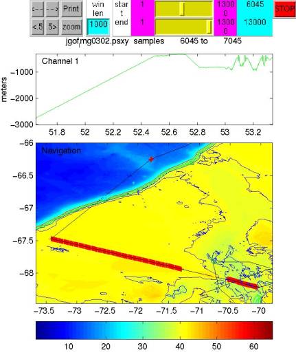
Figure 16. Main window in JGOFSplot MATLAB GUI tool.
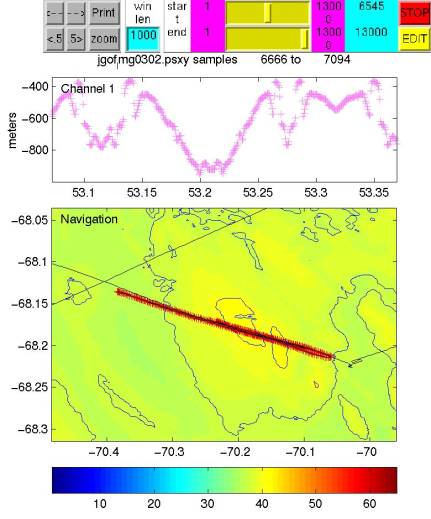
Figure 17. JGOFSplot MATLAB GUI tool zoom window.
function getJGOFS()
% set up parameters to call the JGOFS2mat m-file
% to read JGOFS data
% Tom Bolmer 09/02/03
%%%%%%%%%%%%%%%%%%%%%%%%%%%%%%%%%%%
global CHANNEL_1;
global CHANNEL_2;
global CHANNEL_3;
CHANNEL_1 = [];
CHANNEL_2 = [];CHANNEL_3 = [];
global xnew ynew znew file_name
global savefile_button
global safde_day file_name;
global win_len x
safde_day = 400.0;
win_len = 1;
file_name = input(‘enter filename to read ‘,’s’);
skip=0;
ntraces=1;
% Call m-file to read in data
JGOFS2mat(file_name);
function JGOFS2mat(input)
%
% Tom Bolmer 09/02/03
%
% For use at sea as a VERY crude testing tool
%
% a specialized function for reading the headers of SWD binary files
% To run 1 arguments is needed:
% input: Raw binary data file name.
%%%%%%%%%%%%%%%%%%%%%%%%%%%
global CHANNEL_1;
global CHANNEL_2;
global CHANNEL_3;
CHANNEL_1=[];
CHANNEL_2=[];CHANNEL_3=[];
global ddd dddd hhhh dd hh;
%%%%%%%%%%%%%%%%%%%%%%%%%%%
[CHANNEL_2,CHANNEL_3, CHANNEL_1,dddd,hhhh]=textread(input,’%f%f%f%s%s\n’);
dd=char(dddd);
hh=char(hhhh);
l=length(dddd)
months=[ 0 31 59 90 120 161 192 223 254 284 315 345];
for i=1:l
day(i)=sscanf(dd(i,1:2),’%f’);
mon(i)=sscanf(dd(i,4:5),’%f’);
hour(i)=sscanf(hh(i,1:2),’%f’);
min(i)=sscanf(hh(i,4:5),’%f’);
sec(i)=sscanf(hh(i,7:8),’%f’);
h(i)=(hour(i) + ((min(i)+(sec(i)/60.0))/60.0));
ddd(i)= day(i) + (h(i)/24.0) + months(mon(i));
end
%
mat=1;
%function JGOFSplot(action)
% JGOFSplot
% for JGOFS bathymetry data viewing .
%
% STB 09/02/03
% extensively copied from a file by Jim Doutt of 15 Feb 1994
% ***********************************************
REVIS = ‘03/07/02 11:15’;
global savefile_button NNV
nversio = version;
NNV = str2num(nversio(1:1));
fprintf(‘\n JGOFSplot %s version 1 %s\n\n’,nversio,REVIS);
SAMPLE_RATE = 400.0;
SAMPLE_RATE = 1.0;
FREQUENCY = 1.0 / SAMPLE_RATE;
global CHANNEL_1;
global CHANNEL_2;
global CHANNEL_3;
global x xnew ynew znew file_name;
global safde_day map4 DEPTH;
safde_day = SAMPLE_RATE ;
day = 1;
% graphics initialization
clf reset;
set (gcf,’Units’,’inches’,’position’,[6 5 7 10]);
fig = gcf;
clf;
% Set up some dummy data for plot routines
t = [1 2];
y1 = [0 0];
y2 = 2*y1;
big=length (CHANNEL_1);
x=[1:big];
x=ddd;
smin = x(1:1);
dmax = x(big:big);
% x=x/400.0;
smin = 1;
dmax = big;
g = ‘y’;
start_day_value = smin;
end_day_value = dmax;
win_len = 400;
win_len = 1;
% Set up all pushbuttons
% buttons and display for start day slider
start_day_lab = uicontrol(‘Style’,’Text’,...
‘Units’,’normalized’, ‘Position’,[.38 0.95 .06 .05],... ‘String’,’start’,’backgroundcolor’,’white’);
start_day=uicontrol(‘Style’,’Slider’,...
‘Units’,’normalized’,...
‘Position’,[.52 .95 .20 .05],...
‘Min’,smin,’Max’,dmax,’Value’,smin,...
‘CallBack’,[...
‘start_day_value = (get(start_day,”Value”));’,...
‘set(start_day_valu,”String”,’,...
‘num2str(get(start_day,”Val”))),’],’backgroundcolor’,’yellow’);
start_day_min = uicontrol(‘Style’,’Text’,...
‘Units’,’normalized’,’Position’,[.44 0.95 .08 .05],... ‘String’,num2str(smin),’backgroundcolor’,’magenta’);
start_day_max = uicontrol(‘Style’,’Text’,...
‘Units’,’normalized’,’Position’,[.72 0.95 .08 .05],... ‘String’,num2str(dmax),’backgroundcolor’,’magenta’);
start_day_valu = uicontrol(‘Style’,’Text’,...
‘Units’,’normalized’,’Position’,[.80 0.95 .12 .05],... ‘String’,num2str(get(start_day,’Value’)),’backgroundcolor’,’cyan’);
% buttons and display for end day slider
end_day_lab = uicontrol(‘Style’,’Text’,...
‘Units’,’normalized’,’Position’,[.38 0.9 .06 .05],... ‘String’,’end’,’backgroundcolor’,’white’);
end_day=uicontrol(‘Style’,’Slider’,...
‘Units’,’normalized’,...
‘Position’,[.52 .9 .20 .05],...
‘Min’,smin,’Max’,dmax,’Value’,dmax,...
‘CallBack’,[...
‘end_day_value = (get(end_day,”Value”));’,...
‘set(end_day_valu,”String”,’,... ‘num2str(get(end_day,”Val”))),’],’backgroundcolor’,’yellow’);
end_day_min = uicontrol(‘Style’,’Text’,...
‘Units’,’normalized’,’Position’,[.44 0.9 .08 .05],... ‘String’,num2str(smin),’backgroundcolor’,’magenta’);
end_day_max = uicontrol(‘Style’,’Text’,...
‘Units’,’normalized’,’Position’,[.72 0.9 .08 .05],... ‘String’,num2str(dmax),’backgroundcolor’,’magenta’);
end_day_valu = uicontrol(‘Style’,’Text’,...
‘Units’,’normalized’,’Position’,[.80 0.9 .12 .05],... ‘String’,num2str(get(end_day,’Value’)),’backgroundcolor’,’cyan’);
% button for stating program
start_button=uicontrol(‘Style’,’Pushbutton’,’Units’,’normalized’,...
‘Position’,[.00 .95 .09 .05],’Interruptible’,’on’,’String’,’Start’,... ‘Callback’,’JGOFSdisplay;’,’backgroundcolor’,’green’);
% buttons and display for next full window and 1/2 window
back_button=uicontrol(‘Style’,’Pushbutton’,’Units’,’normalized’,...
‘Position’,[.1 .95 .05 .05],’String’,’<--‘,...
‘Callback’,[’g = “y”;’ , ‘ii = ii - fix(win_len * safde_day);’]);
next_button=uicontrol(‘Style’,’Pushbutton’,’Units’,’normalized’,...
‘Position’,[.15 .95 .05 .05],’String’,’-->’,... ‘Callback’,[’g = “y”;’ , ‘ii = ii + fix(win_len * safde_day);’]);
back2_button=uicontrol(‘Style’,’Pushbutton’,’Units’,’normalized’,...
‘Position’,[.1 .9 .05 .05],’String’,’<.5’,...
‘Callback’,[’g = “y”;’ , ‘ii = ii - fix(win_len * (safde_day / 2.0));’]);
next2_button=uicontrol(‘Style’,’Pushbutton’,’Units’,’normalized’,...
‘Position’,[.15 .9 .05 .05],’String’,’.5>’,... ‘Callback’,[’g = “y”;’ , ‘ii = ii + fix(win_len * (safde_day / 2.0));’]);
% buttons for printing and zooming
copy_button=uicontrol(‘Style’,’Pushbutton’,’Units’,’normalized’,...
‘Position’,[.2 .95 .08 .05],’String’,’Print’,...
‘Callback’, ‘g = “p”;’);
zoomn=uicontrol(‘Style’,’Pushbutton’,’Units’,’normalized’,...
‘Position’,[.2 .9 .08 .05],’String’,’zoom’,...
‘Callback’, ‘g = “z”;’);
% button for STOP
exit_button=uicontrol(‘Style’,’Pushbutton’,’Units’,’normalized’,...
‘Position’,[.92 .95 .08 .05],’String’,’STOP’,...
‘Callback’,’g=”n”;’,’backgroundcolor’,’red’);
edit_button=uicontrol(‘Style’,’Pushbutton’,’Units’,’normalized’,...
‘Position’,[.92 .90 .08 .05],’String’,’EDIT’,...
‘Callback’,’g=”e”;’,’backgroundcolor’,’yellow’);
save_edit_button=uicontrol(‘Style’,’Pushbutton’,...
‘Units’,’normalized’,...
‘Position’,[.89 .85 .11 .05],...
‘String’,’KEEP IT’,...
‘Callback’,’g=”k”;’,’backgroundcolor’,’green’,’visible’,’off’);
% buttons and display for window length in days
day_label=uicontrol(‘Style’,’text’,’Units’,’normalized’,...
‘Position’,[.29 .95 .08 .05],...
‘String’,’win len’,’backgroundcolor’,’white’ );
day_val = uicontrol(‘Style’,’edit’,’Units’,’normalized’,...
‘Position’,[.29 .9 .08 .05],...
‘String’,num2str(win_len),...
‘callback’,[’win_len = str2num(get(day_val,”string”));’],...
‘value’,win_len,’backgroundcolor’,’cyan’);
% Set up areas for figures
beg_y = .10;
beg_y = .10;
del_y = .25;
xa1 = .12; x2 = .90; xtdel = .8; xfdel = .45; xofst = .02; xa1 = .12; x2 = .90; xtdel = .8; xfdel = .45; xofst = .02;
% Figure 2 - channel 2
ax4 = axes(‘Position’, [xa1 beg_y+0.05 xtdel .45],’nextplot’,’replace’,...
‘visible’,’off’,...
‘xticklabel’,’ ‘,’yticklabel’,’ ‘,...
‘xaxislocation’,’bottom’);
ax4_line=image(LONG(1,:),LAT(:,1),DEPTH,’CDataMapping’,’scaled’);
set(ax4,’ydir’,’normal’,...
‘clim’,[-4500 2000]);
ax3 = axes(‘Position’, [xa1 beg_y+0.05 xtdel .45],’nextplot’,’add’,...
‘Visible’,’off’);
ax3_line = plot(t,y1,’EraseMode’,’normal’,’color’,’green’);
ax5 = axes(‘Position’, [xa1 beg_y+0.05 xtdel .45],’nextplot’,’add’,...
‘visible’,’off’,’box’,’on’);
ax5_line=plot(CHANNEL_2,CHANNEL_3,’k’,...
cx.x(5).contours, cy.y(5).contours, ‘b’,...
cx.x(8).contours, cy.y(8).contours, ‘b’,...
cx.x(10).contours,cy.y(10).contours,’g’,...
cx.x(12).contours,cy.y(12).contours,’g’,...
cx.x(15).contours,cy.y(15).contours,’r’,...
cx.x(18).contours,cy.y(18).contours,’c’,...
cx.x(20).contours,cy.y(20).contours,’c’,...
cx.x(24).contours,cy.y(24).contours,’c’,...
cx.x(2).contours, cy.y(2).contours, ‘y’,...
coastx, coasty, ‘g’,... ‘EraseMode’,’normal’);
ylabel(‘Latitude’);
xlabel(‘Longitude’);
axb=axes(‘Position’, [xa1 .05 xtdel .05], ‘nextplot’,’add’,...
‘Visible’,’off’);axbar=colorbar(‘horiz’);
set(axbar,’Position’, [xa1 .05 xtdel .05],’visible’,’on’,...
‘climmode’,’manual’,’clim’,[-4500 2000]);
theLim=[-4500 2000];
relabel(theLim, ‘x’);
ax1 = axes(‘Position’, [xa1 beg_y+del_y+del_y+.05 xtdel .20],’nextplot’,’replace’,’Visible’,’off’);
ax1_line = plot(t,y1,’EraseMode’,’normal’,’color’,’yellow’);
ax2 = axes(‘Position’, [xa1 beg_y+del_y+del_y+.05 xtdel .20],’nextplot’,’replace’,’Visible’,’on’); ax2_line = plot(t,y1,’EraseMode’,’normal’);
TITL=title(file_name);
ylabel(‘meters’);
% JGOFSdisplay()
% function to display JGOFS Bathymetry data.
% Tom Bolmer 09/02/03
% adapted form the below versions
%%%%%%%%%%%%%%%%%%%%%%%%%%%%%%%%%%%%%%%%%%
% MELTPLOT.M
% Plots SAFDE electrical Noise data for the X and Y channels.
% file: meltplot.m
% by: Tom Bolmer
% date: 7/22/97
% for: Alan Chave
% Copied and modeled extensively from a file by Jim Doutt Feb 1994
copied form safdeplot.m
% Stb 7/22/97
%%%%%%%%%%%%%%%%%%%%%%%%%%%%%%%%%%%%%%%%%%
global x CHANNEL_1 CHANNEL_2 CHANNEL_3 xnew ynew znew file_name NNV ddd;
global cx cy coastx coasty map4;
start_day_value=x(1);
end_day_value=x(end);
dev_name = file_name;
x11 = start_day_value;
% Set up the max and min X values to be used in looping through
% the data.
iiend= length(CHANNEL_1) ;
clear start;
clear start1;
if isempty(x11)
start= ‘1’ ;
else
start = x11;
end
set(start_button, ‘Visible’,’off’);
x12=end_day_value;
clear iend;
clear iend1;
iend = length(x);
if isempty(x12)
iend= length(x) ;
else
if iend > length(x);
iend = length(x);
end
end
text (‘units’,’normalized’,’position’,[.025 .9],’string’,’Channel 1’);text (‘units’,’normalized’,’position’,[.025 -.35],’string’,’Navigation’);
ii = fix(start);
% Loop through and do the plotting
while ii < iend
% Find the Max and Min for the data in this window so all% the boxes will have the same axes.
start = fix(ii);
stop = (ii+fix(win_len * safde_day));
yymin = -1 * (max(-1*CHANNEL_1(start:stop)));
yymax = max(CHANNEL_1(start:stop)) ;
if (yymax < 0)
yymax=yymax*.95;
else
yymax=yymax*1.05;
end
if (yymin < 0.0)
yymin = yymin * 1.05;
else
yymin = yymin * 0.95;
end
if (yymin == yymax)
if (yymin < 0.0)
yymin = yymin * 1.05;
else
yymin = yymin * 0.95;
end
if (yymin == 0)
yymin=-.001
end
end
xxmin = x(start);
xxmax = x(stop);
lonleft = (-1 * (max(-1 * CHANNEL_2(start:stop))))-.25;
lonright = max(CHANNEL_2(start:stop))+.25;
latbot = (-1 * (max(-1 * CHANNEL_3(start:stop))))-.25;
lattop = max(CHANNEL_3(start:stop))+.25;
hold on;
set(ax4,’XLim’,[lonleft lonright],’YLim’,[latbot lattop],...
‘visible’,’on’,’clim’,[-4500 2000]);
set(ax3,’XLim’,[lonleft lonright],’YLim’,[latbot lattop],’nextplot’,’add’);
set(ax3_line,’Xdata’,CHANNEL_2(ii:(ii+fix(win_len * safde_day)),:),...
‘Ydata’,CHANNEL_3(ii:(ii+fix(win_len * safde_day)),:),...
‘visible’,’on’,’linestyle’,’-‘,’marker’,’+’,’color’,’red’);set(ax5,’XLim’,[lonleft lonright],’YLim’,[latbot lattop],’box’,’on’);
if (CHANNEL_2(start) < CHANNEL_2(stop))
direction=’normal’;
else
direction=’reverse’; end
set(ax2,’XLim’,[xxmin xxmax],’YLim’,[yymin yymax],’visible’,’on’);
set(ax2_line,’Xdata’,x(start:stop),...
‘Ydata’,CHANNEL_1(start:stop),...
‘linestyle’,’-‘,’marker’,’none’,’color’,’green’);
set(ax1,’XLim’,[xxmin xxmax],’YLim’,[yymin yymax],’Visible’,’off’);
set(ax1_line,’Xdata’,x(start:stop),...
‘Ydata’,CHANNEL_1(start:stop),...
‘linestyle’,’-‘,’marker’,’none’,’color’,’green’);
hold on;
title_str=sprintf (‘%s samples %10d to %10d’,dev_name,fix(ii),fix(ii+fix(win_len * safde_day)));
set (get(ax2,’title’),’string’,title_str); hold off;
% Reset the start slider value
set (start_day,’Value’,ii);
set (start_day_valu,’String’,num2str(ii));
% Wait for an option to be selected
g = ‘stopit’;
while g == ‘stopit’
pause(1); end
% Print the current window
if (g == ‘p’)
print -dps;
g = ‘stopit’;
while g == ‘stopit’
pause(1);
end
end
if isempty(g)
g = ‘Y’ ;
end
% ZOOM in on a selected area
% Use ginput to find the array arguments
while g == ‘z’
clear z1;
clear z2;
[x11,y]=ginput(1);
if isempty(x11)
x11 = ii;
end
cc=find(x < x11);
z1 = x11;
z1 = cc(end);
if (z1 <= 0)
z1=1; end
[x12,y]=ginput(1);
if isempty(x12)
x12 = ii+700;
end
cc=find(x < x12);
z2 = x12;
z2 = cc(end);
% Convert to array arguments from seconds.
z1=fix(z1);
z2=fix(z2);
% Find the Max and Min for the data in this window so all% the boxes will have the same axes.
start = fix(z1);
stop = fix(z2);
yymin = -1 * (max(-1*CHANNEL_1(start:stop)));
yymax = (max(CHANNEL_1(start:stop)));
if (yymax < 0)
yymax=yymax*.95;
else
yymax=yymax*1.05; end
if (yymin < 0.0)
yymin = yymin * 1.05;
else
yymin = yymin * 0.95;
end
xxmin = x(start);
xxmax = x(stop);
lonleft = (-1 * (max(-1 * CHANNEL_2(z1:z2))))-.1;
lonright = max(CHANNEL_2(z1:z2))+.1;
latbot = (-1 * (max(-1 * CHANNEL_3(z1:z2))))-.1;
lattop = max(CHANNEL_3(z1:z2))+.1;
set(ax4,’XLim’,[lonleft lonright],’YLim’,[latbot lattop],...
‘visible’,’on’,’clim’,[-4500 2000]);
hold on;
set(ax3,’XLim’,[lonleft lonright],’YLim’,[latbot lattop]);
set(ax3_line,’Xdata’,CHANNEL_2(z1:z2),...
‘Ydata’,CHANNEL_3(z1:z2),...
‘visible’,’on’,’linestyle’,’-‘,’marker’,’+’,’color’,’red’); set(ax5,’XLim’,[lonleft lonright],’YLim’,[latbot lattop]);
set(ax1,’XLim’,[xxmin xxmax],’YLim’,[yymin yymax]);
set(ax1_line,’Xdata’,x(z1:z2), ‘Ydata’,CHANNEL_1(z1:z2),... ‘linestyle’,’none’,’marker’,’+’,’color’,[1 .5 1]);
set(ax2,’XLim’,[xxmin xxmax],’YLim’,[yymin yymax],’visible’,’on’);
set(ax2_line,’Xdata’,x(z1:z2),’Ydata’,CHANNEL_1(z1:z2),... ‘linestyle’,’none’,’marker’,’+’,’color’,[1 .5 1]);
title_str=sprintf (‘%s samples %10d to %10d’,dev_name,fix(z1),fix(z2)); set (get(ax2,’title’),’string’,title_str);
% button for EDIT
% NOT used for SWD data
% Kept here for future use.
set(edit_button, ‘Visible’,’on’);
g = ‘stopit’;
while g == ‘stopit’
pause(1);
end
if (g == ‘p’)
print -dps;
g = ‘stopit’;
while g == ‘stopit’
pause(1);
end
if (g == ‘y’)
g = ‘Y’;
end
end
if isempty(g)
g = ‘Y’ ;
end
while g == ‘e’
[xnew, ynew, but] = JGOFSgros(CHANNEL_1) ;
xhold=xnew;
yhold=ynew;
xll=length(xnew);
xuse = xll;
xuse = 0;
clear xnew ynew;
for xlll=z1:z2,
xuse = xuse+1;
xnew(xuse)= x(xlll:xlll);
if but(1) == 1
ynew(xuse) = CHANNEL_1(xlll:xlll);
znew(xuse) = CHANNEL_3(xlll:xlll);
else
ynew(xuse) = CHANNEL_2(xlll:xlll);
znew(xuse) = CHANNEL_3(xlll:xlll);
end
end
for xllll=1:xll,
for xlll=1:xuse,
if (xhold(xllll) == xnew(xlll))
if (isnan(yhold(xllll)) == 1)
ynew(xlll) = NaN;
end
end
end
end
title_str=sprintf (‘%s samples %10d to %10d’,dev_name,fix(z1),fix(z2));
title (title_str); hold off;
hold on;
if but(1) == 1
set (ax1,’visible’,’on’,’XLim’,[xxmin xxmax],’YLim’,[yymin yymax]);
set (ax1_line,’visible’,’on’,’Xdata’,xnew,’Ydata’,CHANNEL_1(z1:z2),’marker’,’o’,’color’,’red’);
hold on;
set (ax2,’XLim’,[xxmin xxmax],’YLim’,[yymin yymax],...
‘nextplot’,’add’,’visible’,’off’);
set (ax2_line,’Xdata’,xnew,’Ydata’,ynew,’linestyle’,’-‘,’color’,’blue’);
else
set(ax2_line,’Xdata’,x(z1:z2), ‘Ydata’,CHANNEL_1(z1:z2),’marker’,’+’,’color’,’yellow’);
end
% button for SAVE EDIT
set(save_edit_button, ‘Visible’,’on’);
g = ‘stopit’;
while g == ‘stopit’
pause(1);
end
if (g == ‘p’)
print -dps;
g = ‘stopit’;
while g == ‘stopit’
pause(1);
end
if (g == ‘y’)
g = ‘Y’;
end
end
if g == ‘k’
xll=length(xnew);
xstart=find(x == xnew(1));
for xlll = 1:xll,
xuse = xstart-1+xlll;
if but(1) == 1
CHANNEL_1(xuse:xuse) = ynew(xlll);
if (isnan(ynew(xlll)) == 1)
CHANNEL_2(xuse:xuse) = NaN;
CHANNEL_3(xuse:xuse) = NaN;
end
else
CHANNEL_2(xuse:xuse) = ynew(xlll);
end
end
set(save_edit_button, ‘Visible’,’off’);
g = ‘stopit’;
while g == ‘stopit’
pause(1);
end
end
if (g == ‘p’)
print -dps;
g = ‘stopit’;
while g == ‘stopit’
pause(1);
end
if (g == ‘y’)
g = ‘Y’;
end
end
end
set(edit_button, ‘Visible’,’off’);
set(save_edit_button, ‘Visible’,’off’); end
% END of EDIT Section
if (g == ‘n’)
g = ‘N’;
set(start_button, ‘Visible’,’on’);
end
if (g == ‘N’)
set(start_button, ‘Visible’,’on’);
break
end
hold off;
end
% JGOFSgros()
% STB 09/02/03
% script to remove small spikes from the data
% called by JGOFSdisplay.m
%%%%%%%%%%%%%%%%%%%%%%%%%%%%%%
% splines across spikes. You may want to decrease
% the value of nwid (experiment to see what is best)
% There are also other spline options. Linear may be
% sufficient. % originally written for Alan Chave
function [xnew,ynew,but] = JGOFSgros(e1)
% script to remove small spikes from the data
%%%%%%%%%%%%%%%%%%%%%%%%%%%%%%
global xnew ynew x
x1=1;
d1=1;
clear d1;
clear x1;
clear xnew;
clear ynew;
[xs,ys,but]=ginput(2);
cc=find(x < xs(1));
xl=cc(end);
cc=find(x < xs(2));
xr=cc(end);
nwid= 10;
xhead = xl-nwid;
xr-xl
for i=1:nwid
if but(1) == 1
d1(i) = e1(xhead+i);
d1(nwid+i) = e1(xr+i);
else
d1(i) = e2(xhead+i);
d1(nwid+i) = e2(xr+i);
end
x1(i)= xhead+i;
x1(nwid+i) = xr+i;
xx(i)=x(xhead+i);
end;
for i= (xl+1):(xr-1),
ynew(i - xl) = NaN;
xnew(i - xl) = x(i); end;
return;
%