WinDSSOcK: Winter Distribution and Success of Southern Ocean Krill: Drifter Measurements During 2001

R. Limeburner, R. Beardsley and B. Owens

Woods Hole Oceanographic Institution

Woods Hole, MA 02543 USA

Introduction

A primary objective of this component is to investigate the Lagrangian circulation (fluid particle motion over time) within the Western Antarctic Peninsula (WAP) study area using satellite-tracked surface drifters and isobaric floats.These instruments provide unique information on the horizontal movement of fluid and passive biological particles that cannot be obtained through moored measurements alone.Both Eulerian (fixed) and Lagrangian flow measurements are being made to describe the general circulation.

We plan to deploy about 14 WOCE SVP surface drifters each year during both field years. Six drifters were deployed during the March 2001 mooring cruise, and another eight on the May 2001 broad-scale survey cruise.The initial deployment pattern was to release drifters at each mooring site plus drifters inshore in Marguerite Bay to examine the coastal current in more detail. We do not plan to release any drifters during ice-covered conditions, but to deploy drifters in the spring to study the near-surface flows during ice-free conditions when the large-scale surface-intensified clockwise gyre is thought to exist. 

The WOCE SVP drifter is designed to measure the Lagrangian current using a holey sock drogue centered at 15 m plus sea surface temperature and a proxy to indicate if the drogue is attached.The drifter is located about 20 times per day in the study area, and the position and other data provided daily via Internet by Service ARGOS.For this study, the drifters will feature an ice-hardened surface float to resist being crushed in the ice.Peter Niiler (SIO) and Craig Engler (NOAA) agreed to supply four drifters during 2001 from the Global Drifter Program to this SO GLOBEC program at no cost.

Results of the 2001 Surface Drifter Program

The 14 WOCE SVP drifters were deployed during March - May 2001 at locations shown in Table 1.The drifter deployment locations and tracks are also show in Figure 1 for the large-scale WAP region and in Figure 2 showing the drifter tracks locally in Marguerite Bay. Solid blue circles in Figures 1 and 2 indicate the drifter deployment positions. The drifter tracks shown in Figures 1 and 2 were made during March 20 to August 1, 2001 and are equivalent to 2.3 ?drifter years? of observations. After August 2001 the WAP shelf region was covered with ice and only one icebound drifter was still transmitting data. During the March to August period icebergs, some greater than 1 km wide and 100 m above the sea surface, were observed in the Bay region. Later during this period surface ice was beginning to form. 

 

ID			ARGOS ID	Date	Time Z	Latitude	Longitude
A1			30460	3/26/01	2149	67° 02.400' S	69° 03.000' W
A2			26373	3/30/01	0456	68° 19.920' S	69° 42.109' W
A3			24406	3/30/01	0722	68° 06.162' S	70° 31.797' W
A4			30461	3/30/01	1132	67° 45.216' S	71° 58.957' W
A5			30458	3/31/01	0018	66° 52.331' S	70° 01.168' W
A6			30459	3/31/01	1500	66° 44.543' S	71° 00.012' W
A7			22405	5/3/01	0639	67° 20.809' S	69° 41.768' W
A8			26367	5/5/01	1924	67° 30.800' S	70° 40.600' W
A9			22956	5/7/01	0649	68° 11.000' S	68° 11.000' W
A10			26369	5/8/01	0825	68° 13.600' S	69° 40.400' W
A11			22957	5/16/01	0100	68° 26.123' S	73° 39.205' W
A12			26371	5/26/01	1815	68° 05.300' S	70° 25.000' W
A13			26372	5/27/01	0014	67° 47.285' S	69° 44.784' W
A14			26368	6/1/01	0652	66° 36.668' S	69° 06.450' W

Table 1. Drifter deployment locations and times.

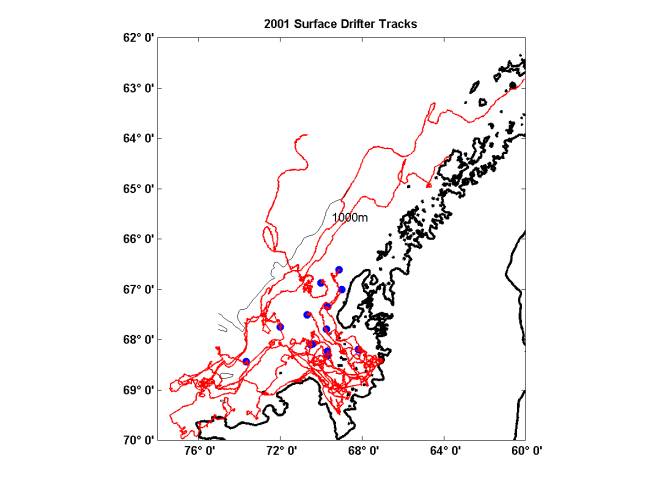
Figure1. Large-scale Surface Drifter Tracks.

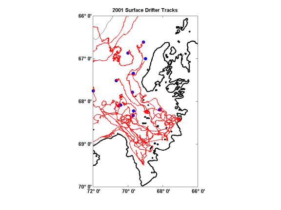
Figure 2. Marguerite Bay Surface Drifter Tracks.

In general the drifter tracks were parallel to the large-scale coastline and bathymetry except at the mouth of Marguerite Bay where the tracks were cyclonically in and out of the Bay. Drifters deployed at the mooring positions initially showed very little mean flow except at mooring A1 located near Adelaide Island where strong near-shore surface inflow to the Bay was observed. The weak mid-shelf surface drifter velocities were surprising due to the strong winds observed during the 2001 cruises. The slow drifter speeds during large wind stress events may be due to the deep surface mixed layer (at least 40 m).For an Ekman layer balance,

f * u * h = Tau/rho.

For Tau = 5 dynes/cm², h = 50m, f = 1.3 10^-4/s, u ~ 1.6 cm/s. Thus, the wind driven response on the open WAP slope may be weak.

The drifter data collected to date suggests that there is surface flow into Marguerite Bay around the southern end of Adelaide Island, with return flow out of the Bay along the northeastern tip of Alexander Island.The surface salinity data supports the idea of a relatively fresh coastal current initially trapped to the topography exiting the Bay along Alexander Island. We hope to deploy future drifters in the mouth of the Bay to further test this idea of a clockwise surface circulation around the Bay. The drifter low pass filtered mean velocities within ¼ degree regions are shown in Figures 3 and 4.

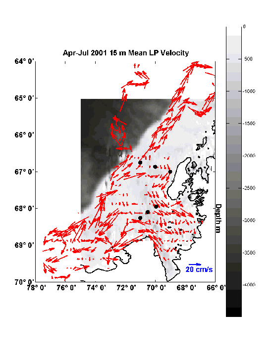
Figure 3. Large-scale mean flow within a 0.25º by 0.25º grid.

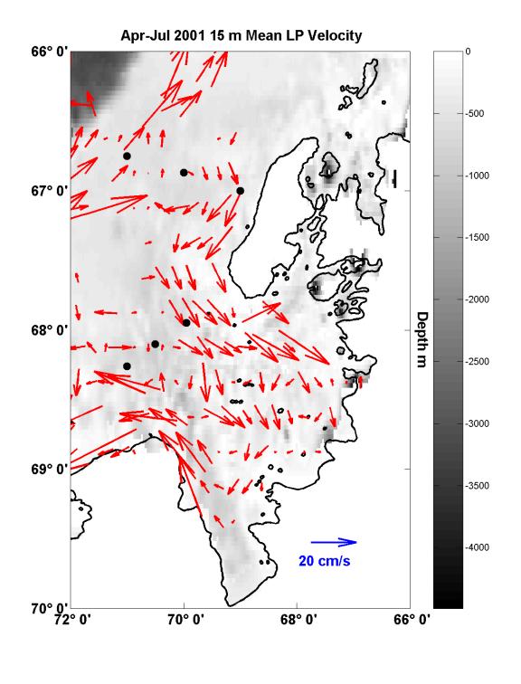
Figure 4. Marguerite Bay mean flow within a 0.25º by 0.25º grid.

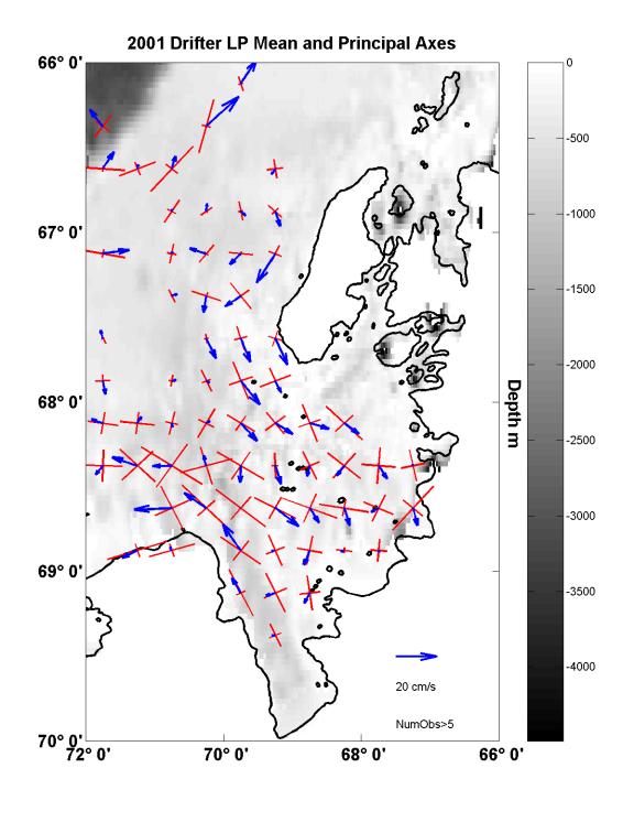
Figure 5. Mean flow and principal axes within ¼ x ½ degree regions.

Similarly, The maximum drifter velocities within ¼ degree regions are shown in Figures 6 and 7.

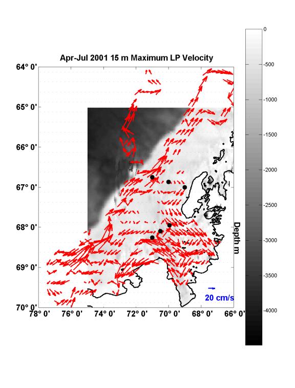
Figure 6. Large-scale maximum drifter velocity within a 0.25º by 0.25º grid.

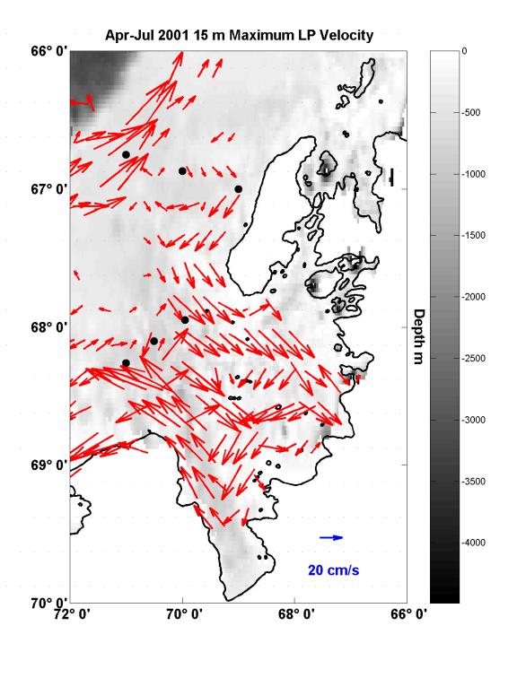
Figure 7. Marguerite Bay maximum drifter velocity within a 0.25º by 0.25º grid.

Drifter Animation

The drifter tracks can most easily be observed from a drifter animation of the 2001 trajectories. Note, for the "flc" animations you will need a movie player capable of reading *.fli/*.flc type movies. The Autodesk Animation Player is one such player.

Lagrangian Time and Space Scales

The Lagrangian autocorrelation function was computed for each drifter velocity component, and then integrated from zero lag to the first zero crossing of the autocorrelation to give a Lagrangian integral time scale. The Lagrangian space scale was then found by multiplying the integral time scale by the rms velocity for each component. The results are shown below.

 

Drifter	ULTS	VLTS	ULSS	VLSS
	Days	Days	Km	Km
1	1.00	1.19	7.5	12.9
2	3.87	1.99	52.1	28.1
3	3.51	1.66	31.7	12.5
4	3.06	1.89	33.2	23.3
5	2.99	2.07	19.3	18.6
6
7	2.82	1.85	15.7	14.5
8	2.92	1.85	32.5	21.5
9	3.19	2.29	24.2	29.1
10
11	2.87	1.47	20.8	12.1
12	2.79	1.67	34	20.6
13
14	2.92	1.05	22.2	7.7

High-Frequency Motion

The above summary is based on the low-pass filtered drifter motion, however, the high frequency of ARGOS fixes per day allow some investigation of the higher frequency drifter motions. A satellite-tracked surface drifter deployed near Broad Scale Station 26 at 19:27 May 5 (yd 125.8105) spent the next 2.91 days makingcounterclockwise loops while slowing moving towards the northeast. This looping motion appears to be inertial.The inertial period at the drifter latitude is 12.99 hours, close to the M2 period of 12.42 hours, so differentiating inertial from tidal motion is difficult with short current records. To quantify this motion, a simple model consisting of a mean current plus inertial component was fit in a least-squares sense to the drifter position data.During this 2.9-day period, this drifter moved in a counterclockwise elliptical path towards the northeast with a mean speed of 3.5 cm/s.The elliptical motion had a major axis of 16.8 cm/s and a minor axis of 10.5 cm/s, with the major axis oriented toward 28 ^ON.After this period, the drifter moved towards the mouth of Marguerite Bay with little high-frequency variability.Further analysis is needed to see if other drifters exhibited near-inertial variability, and if so, with what relationship to the surface wind forcing.