Strongly Nonlinear Internal Waves ...

Strongly Nonlinear Internal Waves on the Australian North West Shelf

Peter E. Holloway
School of Geography and Oceanography
University College, University of New South Wales
Australian Defence Force Academy, Canberra, Australia

E. Pelinovsky and T. Talipova
Department of Nonlinear Waves, Institute of Applied Physics
Russian Academy of Science, Nizhny Novgorod, Russia

Introduction

Soliton-like waves, often called internal solitary waves, are frequently observed to form in the stratified ocean as a result of oscillatory flow over topographic features or from the evolution of large amplitude long internal waves. On the Australian North West Shelf (NWS) a large amplitude semi-diurnal internal tide is generated over the continental slope and propagates shoreward with a wavelength of $\sim 20 km$ and amplitude of a few $10's \, m$ at the shelf break. This long wave evolves into a variety of strongly nonlinear wave forms including internal solitary waves.

In this paper current meter and thermistor observations are presented of varying internal wave forms. Also, numerical solutions of a Korteweg de-Vries model are presented for the evolution of an initially long sinusoidal wave. The model includes varying topography and stratification, the Earth's rotation, cubic nonlinearity and frictional dissipation.

Observations

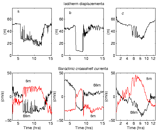
Examples of different internal wave forms are presented as shown by the velocity component flowing across the bathymetry (the dominant wave-propagation direction) and of vertical displacements of isotherms derived from temperature time series at different depths. Measurements are from a NWS location in water 78 m deep close to the shelf break at 19.71^oS 116.14^oE with instruments sampling at 2 min intervals. Additional examples showing soliton-like wave forms are presented by Holloway et al. (1997).

Figure 1a shows a large amplitude wave (peak-trough $\sim 40 m$ in water 78 mdeep) with a downwards shock followed by a number of positive internal solitary waves. At the end of the wave profile when the waveform is again at a crest, negative internal solitary waves are seen. The change in polarity is associated with the dramatic change in the stratification associated with the very large amplitude internal tide. The properties are also revealed in the baroclinic currents (depth average has been removed) at 8 and 68 m depth.

Figure 1b shows a square wave form in displacement and currents where a downward shock of 40 m is followed by an equal upward shock about 2 hrs later. The downward shock produced no short period waves while the upward shock is followed by a large number of oscillatory waves. Figure 1c shows a small number of internal solitary waves following a weak downward jump. The first wave is ``wide" or longer in period than other examples.

Korteweg de-Vries Model

The evolution of internal waves is studied using a Korteweg de-Vries (KdV) model. An initial waveform is defined as a sinusoidal long wave, representing an internal tide, and the wave is allowed to propagate over shoaling topography and through arbitrary density stratification. The model includes the effects of rotation, cubic nonlinearity and dissipation through turbulent bottom friction. Full details are given by Holloway et al. (1998).

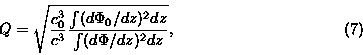
The model is based on the rotated-modified extended KdV equation (reKdV) which is obtained from a perturbation method in second order in wave amplitude and first order in wavelength and is valid when nonlinearity, dispersion and rotation are small. The reKdV equation is,

$\begin{displaymath}\frac{\partial}{\partialx}\left( \frac{\partial \eta}{\parti......^3 \eta}{\partial x^3}\right) = \frac{f^2}{2c} \eta,\eqno(1)\end{displaymath}$

**Figure 1:** Observed time series of vertical displacements of isotherms and corresponding baroclinic cross-shelf currents on the NWS.
$\begin{figure}\epsfxsize=0.95\textwidth %\centerline{\epsffile{Holloway_fig1.eps}}\end{figure}$

where $\eta$ is the wave profile, x the horizontal coordinate, t time, and f the Coriolis parameter. The phase speed of the linear long wave c is determined by the eigenvalue problem (where f is neglected)

$\begin{displaymath}\frac{d^2\Phi}{dz^2} + \frac{N^2(z)}{c^2} \Phi = 0 \eqno(2)\end{displaymath}$

with boundary conditions $\Phi(0) = \Phi (H) = 0$ , normalisation $\Phi _{\max} = 1$ and where H is total water depth and N(z) is the Brunt-Vaisala frequency. The coefficients of dispersion ( $\beta$ ), quadratic nonlinearity ( $\alpha$ ) and cubic nonlinearity ( $\alpha _1$ ) are (Lamb & Yan, 1996),

$\begin{displaymath}\beta= \frac{c}{2} \frac{\int \Phi^2 dz}{\int (d\Phi/dz)^2 dz},\eqno(3)\end{displaymath}$

$\begin{displaymath}\alpha = \frac{3c}{2} \frac{\int (d\Phi/dz)^3 dz}{\int (d\Phi /dz)^2 dz},\eqno(4)\end{displaymath}$

$\begin{displaymath}\alpha_1 = -\frac{\alpha^2}{c} + 3c \frac{\int \left( (d\Phi/dz)^4- (N \Phi/c)^4\right) dz}{\int (d\Phi /dz)^2 dz} +\end{displaymath}$

$\begin{displaymath}+ 3c \frac{\int \left(c(d\Phi/dz)^2 + (N^2\Phi^2/c) -(2\alp...... (d\Phi/dz)\right) (dT/dz) dz}{\int(d\Phi/dz)^2 dz},\eqno(5)\end{displaymath}$

where integration is over the total water depth. T(z) is the first correction to the nonlinear wave mode, given by the solution of

$\begin{displaymath}\frac{d^2T}{dz^2} + \frac{N^2}{c^2} T = \frac{\alphaN^2}{c^4} \Phi + \frac{dN^2/dz}{c^3} \Phi^2 \eqno(6)\end{displaymath}$

with T(0) = T(H) = 0 and the normalised condition $T(z_{\max}) = 0, {\rm where } \Phi(z_{\max}) = 1.$

**Figure 2:** Calculated waveforms, at a depth of $\sim 70 m$ , using different model assumptions with k = 0. (a) kdV model, (b) eKdV model, (c) rKdV model, (d) reKdV model.
$\begin{figure}\epsfxsize=0.5\textwidth\centerline{\epsffile{Holloway_fig2.eps}}\end{figure}$

The effects of slowly varying depth can be included in (1) by introducing a weak source term, as described by Zhou & Grimshaw (1989), defined as,

$\begin{displaymath}Q = \sqrt{\frac{c_0^3}{c^3} \frac{\int(d\Phi_0/dz)^2 dz} {\int (d\Phi/dz)^2 dz}}, \eqno(7)\end{displaymath}$

where values with subscript `₀' are the values at some origin x₀. Quadratic bottom friction with a drag coefficient k can also be introduced. Finally, introducing a change in variable $\zeta (x,s) = \frac{\eta(x,t)}{Q(x)}$ and coordinate $s = \int \frac{dx}{c(x)} - t,$ the model equation becomes.

$\begin{displaymath}\frac{\partial \zeta}{\partialx} + \left(\frac{\alpha\,Q}{c^......eta \vert\zeta\vert= \frac{f^2}{2c} \int \zeta ds. \eqno(8)\end{displaymath}$

Equation (8) is solved numerically with periodic boundary conditions and an initial condition of a sinusoidal internal tide.

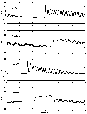
Model Results

Model results are presented for a bathymetric cross-section on the NWS, corresponding to the location of the observations presented in Section 2, using observed stratification from a summer period to define the coefficients in the reKdV model.

The first results presented consider an initial wave of 12 hr period and 2 mamplitude originating in water 500 m deep, although results are not sensitive to the initial water depth as little wave transformation occurs in deep water. Frictional dissipation is also neglected (k = 0). Figure 2 shows the wave forms predicted after the wave has propagated 110 km, to a water depth of $\sim 70 m$ , under different model assumptions. Results are shown neglecting cubic nonlinearity and rotation (KdV model), neglecting only rotation (eKdV model), neglecting only cubic nonlinearity (rKdV model) and including all terms (reKdV model). Solutions without cubic nonlinearity show two solitons forming followed by a train of oscillatory waves. Rotation slows the phase speed of the long wave (latitude is 20^o S). Cubic nonlinearity dramatically changes the form of the solitary waves to produce wide solitons. The full reKdV model produces a nearly square wave form with a train of oscillatory waves.

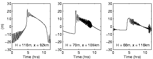
Larger amplitude initial waveforms become unrealistically large as they shoal if dissipation is not included in the model. Figure 3 shows the evolution of a 15 m amplitude wave originating in water 1000 m deep for the same bathymetry and stratification as above using the reKdV model and including dissipation with k = 0.0013. A variety of waveforms result as the wave evolves showing bores, solitons and wide solitons and oscillatory waves.

**Figure 3:** Calculated waveforms from the reKdV model at different depths for an initial wave in water 1000 m deep and amplitude 15 m, with k = 0.0013.
$\begin{figure}\epsfxsize=0.95\textwidth\centerline{\epsffile{Holloway_fig3.eps}}\end{figure}$

Discussion

The use of KdV-type models is one possible tool for developing an understanding of the way nonlinear internal waves can form from an internal tide and how they can evolve as they propagate. Solutions to the model are sensitive to background stratification and initial wave amplitude. Cubic nonlinear effects are dramatic for large amplitude waves and higher order terms could also be important. From theory, background shear flow, not considered here, can also be important in determining the model solutions by changing the values of the coefficients of the KdV model.

References

Holloway, P.E., Pelinovsky, E., Talipova, T., and Barnes, B. A nonlinear model of internal tide transformation on the Australian North West Shelf. J. Phys. Oceanogr., 1997, 27, 871-896.

Holloway, P.E., Pelinovsky, E., and Talipova, T. A generalised Korteweg-de Vries model of internal tide transformation in the coastal zone. Submitted to J. Geophys. Res., 1998.

Lamb, K.G., and Yan, L. The evolution of internal wave undular bores: comparisons of a fully nonlinear numerical model with weakly nonlinear theory. J. Phys. Oceanogr., 1996, 26, 2712-2734.

Zhou, X., and Grimshaw, R. The effect of variable currents on internal solitary waves. Dynamics Atm. Oceans, 1989, 14, 17-39.

About this document ...
1998-08-19