Roger Grimshaw1 and Efim Pelinovsky2
1 Department of Mathematics and Statistics, Monash University,
Clayton, Vic 3168, Australia
2 Institute of Applied Physics, 46 Uljanov Street, 603600
Nizhny Novgorod, Russia
Presented by Roger Grimshaw
In their simplest representation internal solitary waves are nonlinear waves of permanent form which owe their existence to a balance between nonlinear wave-steepening effects and linear wave dispersion. They are now recognised as ubiquitous in nature, and are a commonly occurring feature of coastal seas, fjords and lakes, and also occur commonly in the atmospheric boundary layer (see, e.g., the reviews by Apel et al, 1995 and Grimshaw, 1997). On the theoretical side, it is well-established that nonlinear evolution equations of the Korteweg-de Vries (KdV) type form at least a first-order basis for qualitative modeling and prediction (Grimshaw, 1997).
In general, the study of oceanic internal waves can be separated into three linked components, generation, propagation and decay. Of these three the propagation aspect is perhaps the best understood and indeed will be the focus of this presentation. However, first it is pertinent to make some general comments about the generation and decay processes.
It is widely accepted that in shelf and slope regions the most common generation mechanism is the interaction of the barotropic tide with the continental shelf and slope, resulting in the formation of an internal tide, which in turn can evolve into a structure which allows for the generation of internal solitary waves. In essence, the internal tide can be conceived as a long wave which through a process of local steepening then evolves into a form which supports internal solitary waves of much shorter wavelength. However, this mechanism is certainly not unique, and internal solitary waves can be generated in partially-enclosed regions such as fjords or straits, by current flow over pronounced bottom features, or in fully-enclosed basins through the action of wind stress in tilting the thermocline, followed by relaxation into internal solitary waves.
Direct oceanic observations of decay mechanisms seem to be relatively sparse, but the likely candidates in shallow water regions are bottom friction, and, on the basis of numerical and laboratory experiments, internal wave breaking on a sloping boundary. However, there are certainly other candidates, such as pre-existing turbulence or shear-induced instability.
Next we turn to our main focus, a model for the propagation of internal
solitary waves, but importantly we note that this model can also encompass
some aspects of the generation and decay processes. The model we propose
is an evolution equation of the KdV-type, which incorporates the effects
of background shear, variable bottom topography, both quadratic and cubic
nonlinearity, the earth's rotation and dissipative processes. To describe
the model we we shall at first suppose that the waves are propagating in
the x-direction relative to a background state consisting of a density
profile ![]() and a horizontal current u0(x,z)in
the x-direction, where z is a vertical coordinate. The depth
of fluid is h(x), and here we are assuming that the x-dependence
in the basic state is slowly-varying with respect to the horizontal scale
of the waves.
and a horizontal current u0(x,z)in
the x-direction, where z is a vertical coordinate. The depth
of fluid is h(x), and here we are assuming that the x-dependence
in the basic state is slowly-varying with respect to the horizontal scale
of the waves.
In dimensional coordinates we suppose that the isopycnal displacement ![]() ,
where t is the time, can be represented at leading order by
,
where t is the time, can be represented at leading order by
| (1) |
where the modal function ![]() is defined by
is defined by
| = | (2) | ||
| = | (3) | ||
| = | (4) |
Note that this is an equation in z only, and the slow x-dependence is parametric. This modal equation also defines the linear long wave speed c(x). The system in general defines an infinite system of possible modes, including a barotropic mode, and of these just one is selected, usually the dominant first baroclinic mode. Although we choose to represent the internal solitary waves in terms of the amplitude of the isopycnal displacement, the other fluid variables such as the currents are readily obtained at leading order using local linear long wave theory in the conventional manner. Higher-order correction terms for all fields are also available in principle, and have been explicitly calculated in some special cases.
The amplitude A then evolves according to the generalised Korteweg-de Vries (gKdV) equation,
| (5) |
The independent variables s and ![]() are given by
are given by
| (6) |
while the coefficients ![]() and
and ![]() are
all functions of s. Thus, for instance,
are
all functions of s. Thus, for instance,
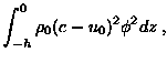
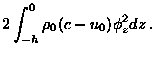
| = | (7) | ||
| = |  |
(8) | |
| = |  |
(9) | |
| = |  |
(10) |
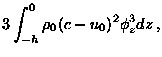
The coefficient ![]() is also available, but is given by a much more complicated expression.
is also available, but is given by a much more complicated expression. ![]() represents dissipation, while f is the local Coriolis parameter.
The derivation of equation (5) is sketched in Grimshaw (1997) (see also
Holloway et al, 1997). Note that s is a time-like variable describing
the evolution of the waves along the ray path determined by the linear
long-wave speed, while
represents dissipation, while f is the local Coriolis parameter.
The derivation of equation (5) is sketched in Grimshaw (1997) (see also
Holloway et al, 1997). Note that s is a time-like variable describing
the evolution of the waves along the ray path determined by the linear
long-wave speed, while ![]() is a phase variable for the solitary waves in a frame of reference moving
with the linear long wave speed c(x). More generally, if
the spatial variability of the background occurs in both horizontal directions,
then s is a coordinate along a ray path defined by c,
is a phase variable for the solitary waves in a frame of reference moving
with the linear long wave speed c(x). More generally, if
the spatial variability of the background occurs in both horizontal directions,
then s is a coordinate along a ray path defined by c, ![]() is a phase variable on this path, while transverse effects can be included
by adding KP-like terms.
is a phase variable on this path, while transverse effects can be included
by adding KP-like terms.
The ``initial'' condition for equation (5) requires specification of ![]() at some specific location, s=s0 (i.e. x=x0)
say. In essence, this is a time series for the amplitude of the baroclinic
mode being considered, and in principle can be obtained from a suitable
data set. However, there is an assumption of ``one-way'' propagation underlying
equation (5), and hence to determine an appropriate initial condition,
it is first necessary to determine that component of the disturbance which
is propagating in the positive x-direction.
at some specific location, s=s0 (i.e. x=x0)
say. In essence, this is a time series for the amplitude of the baroclinic
mode being considered, and in principle can be obtained from a suitable
data set. However, there is an assumption of ``one-way'' propagation underlying
equation (5), and hence to determine an appropriate initial condition,
it is first necessary to determine that component of the disturbance which
is propagating in the positive x-direction.
Although the full equation (5) has not yet been used in an oceanic context
(excepting some very recent work by Holloway et al, 1998), various reductions
have been considered. For example, recently Holloway et al (1997) used
(5) with the omission of the cubic term (![]() )
and the rotational term (f=0) to examine the propagation of internal
solitary wave son the NW shelf of Australia. In general, it is well-known
that a constant-coefficient KdV-model with no dissipation (i.e
)
and the rotational term (f=0) to examine the propagation of internal
solitary wave son the NW shelf of Australia. In general, it is well-known
that a constant-coefficient KdV-model with no dissipation (i.e ![]() with
with ![]() and c constant) will evolve into a finite set of amplitude-ordered
solitary waves (i.e. solitons). Further, the effect of a variable background
on an individual KdV-solitary wave is also relatively well understood.
However, the interplay between quadratic and cubic nonlinearity, variable
background state, dissipation and rotational effects, are issues which
now need to be explored more fully.
and c constant) will evolve into a finite set of amplitude-ordered
solitary waves (i.e. solitons). Further, the effect of a variable background
on an individual KdV-solitary wave is also relatively well understood.
However, the interplay between quadratic and cubic nonlinearity, variable
background state, dissipation and rotational effects, are issues which
now need to be explored more fully.
This presentation will discuss recent work addressing some of these aspects. For instance, we will discuss the role of the cubic nonlinear term in generating kink-like structures, or in the formation of KdV-like solitary waves riding on a background pedestal (Grimshaw et al, 1998b). Also, we will discuss the role of the rotational term in providing an effective damping mechanism through the radiation of small-amplitude waves (Grimshaw et al, 1998a) If time permits we will also discuss recent work on large-amplitude internal solitary waves with vortex cores, which are capable of transporting mass over long distances (Derzho and Grimshaw, 1997).
References