Deployment Procedures
On This Page
2004 Deployment Procedure
Cruise - The Beaufort Gyre Observing System 2004: Mooring Recovery and Deployment Operations in Pack Ice
by J. Kemp, K. Newhall, W. Ostrom, R. Krishfield, and A. Proshutinsky
Woods Hole Oceanographic Institution
Technical Report WHOI-2005-5
Click here for print-friendly PDF version.
Table of Contents
TABLE OF CONTENTS
LIST OF FIGURES
LIST OF TABLES
ABSTRACT
1. PROJECT OVERVIEW
2. MOORING DESIGN
3. METHODS
4. RECOVERY PLATFORM - CCGS LOUIS S. ST. LAURENT
5. TRACTION WINCH
6. PRECISION SURVEY
7. MANEUVERING AND POSITIONING OF VESSEL PRIOR TO RELEASE
8. RECOVERY OPERTATIONS
9. PREPARATIONS FOR REDEPLOYMENT
10. REDEPLOYMENT OPERATIONS
11. CONCLUSIONS
ACKNOWLEDGMENTS
REFFERENCES
List of Figures
Figure 1. JWACS 2004 cruise track (Figure by Sarah Zimmermann), with BGOS moorings locations (stars), and ITP/IMB deployment location (inverted triangle).
Figure 2. BGOS mooring schematic as deployed in 2004.
Figure 3. The Lebus traction winch system installed on the fore deck of the LSL: a) double barreled capstan, b) spooler winch, c) power pack, d) fairlead plate and block, e) remote control box.
Figure 4. Survey plot for mooring B
Figure 5. Top flotation sphere being recovered using the ship's crane.
Figure 6. Wire rope section secured using a Kevlar "Yale" grip. This procedure was used to remove tension from the traction drums when changing reels on the traction winch spooler.
Figure 7. A particularly nasty entanglement of 9 wire rope segments during the recovery of the MMP on mooring C. Amazingly, the instrument was undamaged.
Figure 8. Cluster of glass floats comprising the backup buoyancy being recovered.
Figure 9. Lowering the anchor, BPR, and releases during anchor first mooring redeployment.
Figure10. Top sphere deployment.
List of Tables
Table 1. Summary of BGFE/BGOS 2004 field operations
Table 2. Table of weights and tensions for BGOS mooring A as deployed in 2004
Abstract
Situated beneath the Arctic perennial ice pack, the principal components of the Beaufort Gyre Observing System are three deep-ocean bottom-tethered moorings with CTD and velocity profilers, upward looking sonars for ice draft measurements, and bottom pressure recorders. A major goal of this project is to investigate basin-scale mechanisms regulating freshwater and heat content in the Arctic Ocean and particularly in the Beaufort Gyre throughout several complete annual cycles. The methods of recovering and re-deploying the 3800 m long instrumented moorings from the Canadian Coast Guard Icebreaker Louis S. St. Laurent in August 2004 are described.
In ice-covered regions, deployments must be conducted anchor-first, so heavier wire rope and hardware must be incorporated into the mooring design. Backup buoyancy at the bottom of the mooring is advised for backup recovery should intermediate lengths of the mooring system get tangled under ice floes during recovery. An accurate acoustic survey to determine the exact location of the mooring, adequate ice conditions, and skilled ship maneuvering are all essential requirements for a successful mooring recovery. Windlass (or capstan) procedures could be used for the recovery, but a traction winch arrangement is recommended.
1. Project Overview
The Beaufort Gyre has been characterized in the past as the region of “relative inaccessibility” in the Arctic Ocean because of the difficulty of accessing the area by icebreaker due to heavy ice conditions and by airplane due to its remoteness from the mainland. As a result, the area is one of the most poorly sampled regions in the Arctic Ocean. In 2002, the National Science Foundation (NSF) Office of Polar Programs recognized the great importance of the Beaufort Gyre in the fresh water balance of the Arctic Ocean and funded the “Beaufort Gyre Freshwater Experiment (BGFE): Study of fresh water accumulation and release mechanism and a role of fresh water in Arctic climate variability” (Principal Investigator, Andrey Proshutinsky). The major goal of this project was to investigate basin-scale mechanisms regulating freshwater content in the Arctic Ocean and particularly in the Beaufort Gyre throughout a complete annual cycle. As part of the field experiment for this project, three bottom-tethered moorings were deployed with CTD and velocity profilers, upward looking sonars for ice draft measurements, and bottom pressure recorders, and four expendable surface buoys with CTDs during a Joint Western Arctic Climate Study (JWACS) cruise on the Canadian Coast Guard Icebreaker Louis S. St. Laurent (LSL) in August 2003 (Ostrom et al., 2004).
However, given the importance of this region for Arctic climate studies, it was desired to investigate interannual and longer variability, so that it was necessary to continue acquiring the same data for several years, although the observational program supported by NSF would end with recovery of the moorings in 2004. In 2004, WHOI’s Ocean and Climate Change Institute provided the support to redeploy the three moorings in order to continue monitoring freshwater and heat content in this climatically sensitive region of the Arctic Ocean, thus establishing the Beaufort Gyre Observing System (BGOS).
In August 2004, the sites were revisited, the moorings were recovered, data were retrieved from the instruments, the hardware and sensors were refurbished, and the systems were redeployed at the same locations again from the LSL during a JWACS cruise (Figure 1). In addition, a prototype Ice-Tethered Profiler (ITP) buoy was deployed in combination with an Ice Mass Balance (IMB) buoy. The times and locations of the 3 recovery and deployment operations are given in Table 1. More information on the BGFE/BGOS project, including the scientific motivation, publications, descriptions of methods (instruments and modelling), field operations (including dispatches from each of the cruises), historical and acquired data, and a “History of Arctic Exploration and Scientific Discovery” are available on this website.

In 2004, NSF granted a 5-year proposal “The Beaufort Gyre System: Flywheel of the Arctic Climate?” so that all the moorings that are recovered in 2005 with support of the WHOI Ocean and Climate Change Institute, will be maintained until 2008 with NSF support and investigation of the Beaufort Gyre system will continue.

2. Mooring Design
The bottom-tethered moorings which were deployed in 2003 are described thoroughly in Ostrom et al. (2003). Briefly, each mooring consists of a top sphere providing 2500 lb of buoyancy and housing an Upward Looking Sonar (ULS) and Benthos transponder. The length of each mooring was individually adjusted so that the top sphere would be located at 45 m, however only one of the three moorings actually ended up close to the correct depth while the other two ended up deeper than intended due to uncertainties in the bottom depth and incorrect wire lengths. The ULS acquires ice draft data, while the transponder is used for remotely determining the location of the mooring by performing an acoustic survey.

Below the top sphere and chain bridle, a 2000 m segment of wire rope supports a McLane Moored Profiler (MMP), which acquires seawater temperature, salinity and velocity profiles approximately twice every two days between about 50 and 2000 m. Where the upper sphere was deeper than intended, the upper limit of the MMP is also deeper. Below the MMP, various wire rope segments and glass floats were distributed to fill in the mooring length, reduce tension on the wire during deployment, and provide backup buoyancy for recovery.
On one mooring (A), a McLane Research sediment trap was installed at 3000 m depth for a biogeochemical particle flux study. At the bottom of each mooring is a 3800 lb anchor, with mount for a Bottom Pressure Recorder (BPR) to measure the pressure of the entire water column. The BPR is attached to a set of dual releases which are suspended above the anchor. Triggering one of the two releases with an acoustic pulse causes the entire system (except anchor) to float to the surface where it can be recovered.
On all the moorings, the glass flotation spheres were redistributed differently along the mooring in 2004 compared to 2003, in order to reduce tangling of the wire on recovery. A schematic of the BGFE mooring design as redeployed in 2004 is presented in Figure 1.
3. Methods
The method of deploying and recovering bottom-tethered moored instruments in Arctic ice-covered waters from air supported landings and using divers for recovery was described by Aagaard et al. (1978). Before icebreaker vessels were able to regularly penetrate the perennial ice pack, these air supported operations (also employed by Institute of Ocean Sciences (IOS), Canada) provided the only means to regularly revisit moored sites, and are still utilized today for annual maintenance of North Pole Environmental Observatory systems (http://psc.apl.washington.edu/northpole). In this technical report, we describe the methods of recovering and re-deploying instrumented deep-ocean bottom-tethered moorings within the Arctic perennial ice pack from icebreakers without diver assistance.

In the Arctic ice pack, it is not normally feasible to deploy bottom-tethered moorings in the traditional manner of spooling out the entire mooring on the surface and deploying the anchor last. Consequently, the anchor must be deployed first, which increases the working tension during deployment. As a result, the BGOS moorings are 8 designed with: 1) heavier gauge wire rope (5/16”) for increased strength, and 2) backup flotation at the bottom to allow for the entire mooring to be recovered if the mooring parts during deployment (or anytime prior to recovery). The backup buoyancy also allows the mooring to be recovered from the bottom end if the upper mooring becomes tangled in ice floes during recovery.
Table 2 lists the design weights, lengths and buoyancies of mooring A as deployed in 2004, and estimated tensions during deployment and recovery. Note that the minimum backup buoyancy at any time during deployment is always greater than 500 lb. Static tension varies from as much as 4000 lb to as little as 1700 lb during the deployment as each item of equipment and flotation are attached. Tension during recovery is always less than 1600 lb.
4. Recovery Platform - CCGS Louis S. St. Laurent
Unlike most mooring operations conducted on UNOLS vessels where the mooring deployment and recoveries are performed from the stern of the vessel, mooring operations on the LSL are conducted from the foredeck of the ship. The work area is equipped with a starboard side A-frame and two stiff boom cranes located on either side of the foredeck, each capable of lifting heavy gear out of the water. The deployment cruise on the LSL in 2003 utilized the ships windlass to deploy the BGOS moorings, but this technique proved to be rather slow and labor intensive, and would be more so during recovery operations. Consequently, a special traction mooring winch system (manufactured by the Lebus company in England) and custom fairlead plate were installed on the ship for use in conjunction with the ship’s cranes and A-frame in the recovery and re-deployment of the moorings in 2004 (Figure 3).
5. Traction Winch
The Lebus traction winch system consists of three primary components: the double barreled capstan, spooler winch and power pack. The function of the winch system allows mooring wires and ropes to be deployed and recovered utilizing a double 9 headed capstan acting as a traction winch in conjunction with a tension spooling winch that provides constant back tension on the mooring wire and supports individual wire and rope mooring segments reels.
The double barreled capstan is the load bearing or hauling segment of the winch system (high tension component), and the spooler winch is the mooring wire and rope delivery system (low tension component). In haul mode, this system operates by the capstan winch pulling the mooring wire (with constant tension) from the spooler winch.

The capstan winch has two capstan barrels positioned horizontally one over the other. There are two fair lead gates located at the front and rear of the winch through a b c d e 10 which the mooring wire enters and exits. The free end of the mooring wire is guided through the front fairlead gate (low tension side), wound around the two capstan barrels with typically 5 to 6 wraps, and passed out through the rear fair lead gate (high tension side). The axial ordination of the upper barrel is important in maintaining adequate separation between the wire wraps. The separation between each wrap can be adjusted by activating a manual hydraulic control pump that pivots the upper capstan barrel horizontally, causing the wire wraps to migrate towards the desired inner or outer edge of the barrels. The capstan winch is operated from a remote control box. This control box is fitted with an emergency stop button and a toggle control that allows the capstan barrels to operate at infinite speeds. The winch’s operating capacity is 7000 lb at 30 fpm.
The spooler winch is a hydraulically powered reel stand that is controlled separately from the capstan winch. This winch is designed to support wooden wire and rope storage reels and to provide a haul in line tension up to 250 lb. The spooler winch should nominally maintain between 125 to 150 lb of back tension in order to keep the wraps tight on the capstan barrels. The spooler is generally positioned approximately 10 ft from the low tension side of the capstan winch. This is to allow for adequate working area between the two pieces of equipment in order to connect and disconnect wire and rope mooring segments. The capstan and spooler winches are powered by a 400 volt, 3- phase, 60Hz electric hydraulic power pack.
Traditionally, moorings winches have been configured with single large drums. All of the mooring wire and rope shots are pre–wound for deployment and off spooled following a mooring recovery from a single drum. The Lebus winch system saves substantial ship time by not having to handle the mooring wire twice. These components can be compressed and fouled on a single drum due to high mooring tensions and are often damaged from kinking. Mooring wire and ropes that are recovered and wound onto wooden storage reels are undamaged because of the Lebus spooler winch’s low hauling tensions, making it possible to redeploy these components.
The Lebus winch system requires three personnel that are thoroughly trained in the winch’s operation and have a familiarity with the mooring components that are going to be deployed or hauled. These technicians are the capstan, slew and spooler operators.
The capstan operator must have a clear understanding of the following points:
a. The double barreled capstan has a greater line pull than the spooler winch.
b. The double barreled capstan has in most cases has a hauling potential that could break the mooring wire or rope.
c. The capstan winch will hold the load only as long as there is an opposing minimum load of 125 lb on the low tension side of the winch. The capstan operator’s responsibilities entail the following:
a. Controlling the speed and direction of haul in and pay out of the mooring wire.
b. Ensuring that the capstan winch’s fair lead gates are positioned correctly.
c. Verifying that personnel are clear of the rotating capstan barrels.
The slew operator’s working area is between the capstan winch and the spooling winch. This operator’s responsibility is to keep constant observation of the wire or rope wraps that are bent around the capstan barrels and adjusting the axial angle of the upper capstan barrel so that the wraps are equally spaced. In addition, the slew operator’s responsibilities include:
a. Monitoring the retarded tension from the spooler winch.
b. Confirming that the correct mooring components are being passed around the capstan winch.
c. Opening and closing the low tension gate.
d. During mooring pay out, ensuring that all hardware terminations are wrapped prior to passing around the capstan winch.
e. Securing a stopper line to the loose end of a deployed mooring wire during reel changes.
The spooler operator should be efficient in reel transfer operations and be familiar with the mooring components to be used in the mooring. The spooler operator’s responsibilities include the following:
a. Checking that the correct mooring wire or rope segment is on the winch.
b. That the storage reel secured to the winch has been shafted correctly, in order to prevent the reel from coming lose from the winch drive pin spinning free causing uncontrolled mooring wire slack on the capstan drums.
c. Verifying that personnel are clear of the spooler winch prior to capstan operator starting payout or hauling in.
d. Keeping the line in setting on the spooler winch high enough to provide adequate back tension on the mooring wire or rope against the capstan drums to prevent slippage.
e. The spooler operator must never shift the winch into the pay out or neutral mode while there is a load on the high tension side of the capstan winch.
6. Precision Survey
During the time that a mooring system falls to the seafloor when deployed, it is subject to some drift along the way due to currents and wire angle. This is especially true for anchor last deployments where the mooring system is stretched out horizontally during the operation, so that the system will typically fall around 15% of length of the mooring away from the anchor drop site. For anchor first deployments, this effect is much less since the mooring is already stretched out vertically, and the anchor has less distance to fall. The BGFE/BGOS moorings were designed for the top float to be only 50 m from the surface when installed, and were deployed anchor first, so that anchor would only have to drop less than 100 m when let go during the deployment. Consequently, it was expected that the locations where the moorings were let go during deployment would be very close to the locations where the anchors were actually positioned.
However, for recovery operations in sea ice, it is extremely important to know the exact location of the mooring, so the system is not released under ice floes, but rather in open water areas. Therefore, a close range acoustic survey on transponders mounted on the mooring was performed prior to each recovery operation. Basically, the survey consists of measuring slant range response times of acoustic pulses from a transponder on the mooring from several different locations around the expected mooring site, and determining the intersection of the circles.
The survey begins by selecting a location near (typically within 1 km) of the mooring site and hanging an acoustic transducer over the side of ship, between 5 to 10 m below the sea surface. Markings on the transducer cable may be used to facilitate determining the actual depth of the transducer, which is needed for the calculations. On the BGOS moorings, Benthos transponders are mounted on the top flotation spheres for survey purposes, but the Edgetech acoustic releases at the bottom of the mooring could also be used as transponders for the survey. Using the transducer deck unit (in our case an Edgetech model 8011), an interrogate frequency pulse is sent to the transponder, which responds with a reply frequency pulse. The time between pulses (travel time) is measured by the accurate time clock in the deck unit, and displayed (or may be recorded digitally). Simultaneously, the location of the survey point must be recorded.
Ideally, the location of the survey point is the exact location where the interrogate transducer is positioned. Here, we obtained GPS locations from the ship’s bridge, so that there was some offset (on the order of 20-30 m) between the recorded and actual transducer locations. This discrepancy will result in some error in the measured travel time, and will generally reduce the precision of the triangulated mooring location.
An acoustic survey software program developed at WHOI by Arthur Newhall is used to perform the calculations for determining the actual mooring location using a least squares estimation algorithm on the intersection of the data from the survey points. In addition to the survey point response times, the program requires entries for the depth of the shipboard transducer, depth of the mooring transponder and speed of sound of the seawater; sound speed profiles were obtained from a CTD cast. On the BGOS moorings, the transponders were between 50 and 80 m deep, and the mean speed of sound in the upper layer was approximately 1460 m/s.
Using the travel times (which are slant times between the transducer and the transponder), depths, and speed of sound, the slant times are converted into horizontal ranges which are plotted as circles around the respective survey locations. The least squares estimate of the intersection determines the actual mooring location. The estimates used for the speed of sound and transponder depths can be adjusted to improve the intersection of the circles. Sometimes survey locations too close to the mooring site can produce erroneous circles, probably because the return time is too quick for the deck unit so that it detects reflections.

Uncertainties associated with the location, speed of sound, and transponder depths added up to an apparent error of approximately 20 m in the range of any single survey point. However, by taking multiple survey points, the statistical error of the triangulated estimate is reduced. The error in the location was the largest contributing factor, and could be reduced by obtaining location directly over the shipboard transducer using a hand-held GPS.
During the 2004 field operations, a full survey was not conducted at mooring A but a single range was taken 100 m from the mooring which coincided with the expected location. The survey from mooring B (Figure 4) indicated the actual mooring site was 44 m away from the expected location. For some unexplained reason, the survey from mooring C indicated that the actual mooring site was 183 m due west from the mooring site.
7. Maneuvering and Positioning of Vessel Prior to Release
After determining the exact location (latitude and longitude) of the mooring from the acoustic survey, the ship traveled to the site and was positioned directly overhead. A visual examination was then performed to establish both the thickness of ice in the area, and if there were any leads (lanes of open water) present. Set and drift calculations were then performed to see how natural forces (wind and current) affected the vessel‘s positioning over time. This is very important in determining the ship’s overall movement in relation to the mooring’s position.
The ice concentration on the site then determined the next course of action. At every site, the ice concentration (from analysis by Environment Canada) was 9/10ths or greater. Looking at RADARSAT satellite imagery and by visual inspection, the ice observer on board determined whether the ice was first year, second year, or multi-year and estimated the total mass at the different sites. If necessary, the ship would spend up to 2-3 hours breaking up the ice, attempting to create an open pond sufficient for the top sphere (buoy) of the mooring to surface when released.
During all three mooring recoveries the use of the ship’s “Wartsila Bubbler System” was essential to keep the ice clear from starboard (where the A-frame used for hauling the moorings was located) and for positioning the ship without having to use excessive engine and thruster power. Typically used for reducing ice friction during ice breaking, the bubbler system consists of two large air compressors capable of outputting air at 6 m3 s-1 at 190 kPa through various vents located along the forward and lateral waterline on both the port and starboard sides. At any given time, the operator can activate different groups of vents in order to focus the bubblers on specific areas. The use of the bubblers was very important to the success of the mooring operations, especially in the heaviest ice conditions.
At mooring site A, the ice was mostly first year, and there were many leads and a few open water ponds. As it was the first site that we visited on the cruise, it was the first opportunity to put the tactics described above to use. After several hours of breaking the ice, it was found that, because of the leads present, the ice would spread out to create open water. Once it was concluded that a large enough pond was present (for at least 3 minutes), the decision to release the mooring was made. The position of the mooring at the time of release was directly underneath the vessel. It took approximately 30-40 seconds for the buoy to surface. By the time the buoy surfaced, the ship had moved far enough for the buoy to surface off of the starboard by about 20-30 meters.
The differences found at site B were: the ice was both first year and second-year, there were fewer leads, and there were fewer ponds visible. This changed the tactics slightly. The captain decided to spend more time with the survey, breaking up the ice, and determining set and drift, to make sure that it was possible to create a patch of open water. Because there were less leads present, it took more preparation time leading up to the release of the mooring.
At site C there were no leads present, it was all multi-year ice, and there were no visible open water ponds. After many hours of breaking ice, still no leads or open water areas were created because there was more ice present, no leads, and no wind to distribute the crushed ice. An adaptation was made when the mooring was ready to be released. Instead of keeping the mooring underneath the vessel as in site A and B, it was decided that the mooring would be positioned at the stern. The release command was given and the Captain backed the ship hard astern to clear the ship of the surfacing buoy, and to create the open water necessary for the recovery.
The main conclusions drawn are that heavy ice concentrations can be overcome with patience and by taking the essential steps described above to create an open water area exactly where needed. Without open water, there is a risk that the buoy could get trapped underneath a larger ice flow and make it virtually impossible to recover the mooring. Under the most severe conditions, as encountered at mooring site C, the need to position the mooring at the stern while backing the ship is critical to create an opening. Without that adaptation there simply would not be enough time or space for the mooring to surface.

8. Recovery Operations
Due to the high free board of the LSL fore deck above the water (10 m), it would be extremely difficult to attach to surfaced mooring components with conventional pickup poles and hooks. Some traditional methods used from ships with a high freeboard for attaching a recovery line were either done using a small boat or by lowering a person in a man basket. Both methods are time consuming and labor intensive and the launching of the small boat would be dependent on the ice conditions on the day of recovery. When working in the ice there is no sea state induced motion, so at the suggestion of the Boatswain, we adopted a method using an open-end recovery hook and steering tag line.
The recovery hook was suspended on a 3-meter wire pennant from the block on the crane. Once the mooring sphere had surfaced, the Captain maneuvered the ship to a point where the sphere was directly under the position of the cranes on the fore deck. The open ended hook was lowered and skillfully positioned using the steering tag line into the pickup point on the sphere (Figure 5). Once hooked, the sphere was hoisted up out of the water. This hooking method relied on skillful coordination between the person steering the recovery hook and the crane operator but proved to be a reliable and a less time consuming method of retrieving gear out of the water in ice covered conditions.
Once hoisted out of the water, the crane maneuvered the sphere into a position directly under the A-frame. A vertical chain stopper with a safety hook attached to the bitter end (previously suspended from a pad eye on the A-frame) was then snapped into a sling link (disconnect point) under the sphere. The load was then transferred to the chain stopper, and the buoy was disconnected and craned to a position on the deck of the ship where it was secured.
The traction winch tag line was then shackled into the stopped off sling link and the winch then took the load of the mooring so the vertical chain stopper safety hook could be removed. At this point, the mooring wire was hauled up far enough for the removal of the upper MMP bumper stop. Once the bumper was removed, the winch began hauling in the first shot of 1995 m of 5/16” wire rope. When the termination of the first shot of wire rope reached the winch, a preassembled 1/2" chain bridle shackled to the winch base was used to secure it, and the load was transferred to a “Yale Grip” which was shackled to the chain bridle, thus taking all the weight away from the winch drums (Figure 6).
This allowed the winch tag line to be unshackled and the spool containing the tag line to be replaced by a collapsible wire coiler. The wire rope would not be reused on any deployments therefore the coiler allowed ~300 meters of 5/16” to be bundled and stored then disposed of at WHOI. The coiler was only used on the recovery of A. On subsequent mooring recoveries, the wire was wound on the empty spools used for the previous deployment and stored on deck. When the recovery process continued, the termination was wrapped in canvas to protect the winch drums while spooling around the drums of the winch.

At the bottom end of the 1995 m shot of wire rope, the MMP was retrieved resting on a second bumper stop. The MMP was hauled in until the vertical chain stopper could hook into the sling link just below the bumper stop. The winch then payed out enough wire rope to transfer the load and position the MMP and bumper stop on the deck to be disconnected. Once the MMP was safely on deck, the load was shifted back to the winch and the remaining length of the 1995 m shot of wire was brought in.
However, due to the backup flotation positioned at the bottom of each mooring and spring effect of the wire upon release, each mooring typically had some entanglements (wuzzles) in the wire rope which complicated the recovery. Where this occurred, the mooring had to be stopped off while portions of the wires were sorted and brought on deck (sometimes manually, at other times in bites using the vertical chain stopper, and once using the ship’s windlass as a secondary winch). At times,

entanglements of more than 5 different shots of wire were shackled together and wound around the winch at once, while making sure that they did not tangle while passing through each block. Once most of the wire shots above the flotation spheres at the bottom had been recovered, the next task was to recover the spheres.

The glass spheres also snarled in large bunches (Figure 8) and sometimes were wedged just underneath the ice. In order to recover the spheres without putting too much strain on the wire, it was decided to slowly pay in the winch while the ship slowly traveled toward the direction of the wire. In other words, the captain went to the spheres instead of trying to pull the spheres to the ship. This method proved to be extremely effective and necessary in order to recover this section of the mooring safely. Because of the enormous snarls, the spheres were literally caught up in the ice and required a vertical lift instead of a horizontal drag.
When the floats were reached, an open-end recovery hook and steering tag line was used to attach to the cluster. The ship’s crane was lowered, and the Boatswain hooked onto a link of chain, a shackle, or a pear ring, then raised the cluster to the Aframe. The vertical chain stopper was used to hook into a termination of wire below the balls in order to stop off the mooring so the floats could be disconnected and brought onto the deck.
The final systems to be recovered were the dual releases and BPR (although once they were recovered before all of the backup buoyancy was retrieved due to the entanglements). The BPR was mounted on the anchor and chained to one of the releases at the bottom of the mooring. When the release command was given, the BPR was pulled from the anchor mount and ascended along with the rest of the mooring. Eventually the releases and BPR were brought to the surface away from the ice pack and secured to the vertical chain stopper. The wire was slackened, the termination was disconnected, and the load was transferred to the ship’s crane. The crane then moved the releases and BPR to the deck of the ship therefore ending recovery operations.
At critical points during the recovery, especially when instruments were at the surface, the ship’s bubbler system was used to clear broken ice fragments away from the starboard side.
9. Preparations for Redeployment
Once each mooring had been recovered, the next phase of the operation was to dump data, turn around the recovered mooring flotation packages, check releases, and prepare the instrumentation for redeployment. A full day between recovery and redeployment operations was occupied in the mooring refurbishment while the ship occupied CTD/Rosette stations.
Mooring Systems:
Even though each mooring was in an area without a significant sea state, thus reducing cyclical wear, the decision was made previously that the wire and hardware would not be reused primarily due to the tension during deployment and release during recovery. Therefore, complete new sets of wire and hardware were brought for each mooring.
Each mooring had a total of 52 glass floats (12 sets of 4 and 2 sets of 2) so there were numerous sets of hardware to change. After recovering the glass flotation balls the previous day, each set was separated and the used shackles and pear rings were discarded. Each set required complete new sets of 1/2" trawler chain (4m lengths) and 3/8” hardware (bolts, fender washers, locks, and nyloc nuts). Two technicians using a “hard hat” table setup and impact wrenches performed the process in roughly 3-4 hours.
Six releases also needed to be inspected. Ones that passed inspection and operation test on deck were turned around and redeployed. Each of these required two new anodes and a new chain bridle with two new links. However, two spare releases were utilized on the redeployment in lieu of releases with problems (one had a power problem, and another had a leaky acoustic transducer).
Instrument Systems:
Upon recovery, data was retrieved from the MMPs, ULSs, and BPRs, and the instruments were cleaned, evaluated and prepared for redeployment. Fortunately, none of the instruments were damaged, so all could be reused after maintenance. Additionally, in order to check the drift of the temperature and conductivity sensors on the MMPs, in situ calibrations were performed using a cast of the IOS SeaBird CTD/Rosette as a reference.
Data was dumped from each MMP and a preliminary analysis was performed to ensure that the instrument operated properly, and that the acquired data looked reasonable. The FSI EMCTD on the MMP was removed, configured with an independent power source, attached to the IOS CTD/Rosette frame, and configured to acquire data during a cast. This data was compared to the IOS CTD data, and if the differences were within stated accuracies, the EMCTD was remounted onto the MMP. Otherwise a spare previously calibrated EMCTD was substituted. The MMP ACMs were inspected for leakage, and if the data looked reasonable was also reused. The remainder of the MMP was refurbished for redeployment by installing a new drive roller, spring, and battery, and was reballasted for weight differences between the old and new battery packs (and old and new sensors, when necessary) and to reduce the difference in current drawn by the instrument between up and down casts (to enhance battery duration).
All of the ULSs and BPRs recovered in 2004 acquired complete datasets that looked reasonable. The battery pack for each ULS was replaced and since every anode was significantly they were replaced. The battery packs and antifouling devices were replaced in the BPRs.
After rescheduling (see Ostrom et al., 2004 for example), the instruments were ready for redeployment.
10. Redeployment Operations
Deployment operations began in the morning. In order to prevent freezing, the instruments were stored inside until just before arriving on site. While the ship calculated drift and cleared space in the ice (time varied for each mooring), the ULS and transponder were mounted to the top float and the BPR was installed on the anchor.
Each mooring was deployed anchor first using the Lebus winch. The first phase of each mooring deployment required the attachment of the dual Edgetech releases to the anchor. The ship’s crane was used to both raise the releases into place over the anchor, and to lower the anchor outside of the A-Frame where the top of the 3m shot of trawler chain was secured to the vertical chain stopper (Figure 9).
The crane then hooked into the first set of glass balls that were staged on the deck and lowered them until the bottom pear ring could be shackled into the top of the trawler chain. The load was shifted to the ship’s crane and the vertical chain stopper was disconnected. The load was lowered until the vertical chain stopper was connected into the pear ring at the top of the balls. The crane then connected into a second set of glass balls and the process was mimicked until all 12 sets of balls were connected onto the mooring array. In order to reduce snarling of the wire rope on future recovery operations, the glass floats were re-distributed on the redeployed mooring system so that all of the significant backup buoyancy was directly above the anchor. In other words, 12 sets of 4 were at the bottom, and 2 sets of 2 were at the top.

After the flotation spheres were in the water, the next four shots of 5/16” wire to be deployed were all equal to or less than 100m in length. Therefore, the smaller shots of wire were pre-connected to the 500m shot that was to be deployed after the smaller shots. This enabled the mooring deployment to proceed smoothly without having to stop the mooring off using the Yale-grip bridle (described above) when a small shot of wire had to be added. It is extremely important to note that six wraps of 5/16” wire were necessary around the Lebus heads in order to ensure proper tension on the wire while both recovering, and deploying the moorings. Also, before a termination went around the winch, it was wrapped in canvas for protection.
After the first shot of 500m of wire, a PARFLUX sediment trap with 0.5 m2 aperture was added to mooring A (but not B or C) at 3000 m depth. The same method of using the vertical chain stopper and the ship’s crane was used in order to add this instrument.
After two more 500 m shots and one 10m shot of wire were added to the mooring, the 1995 m shot was next. WHOI technicians and the ship’s crew were all needed to add the large shot of wire. Because of hydraulic problems on the spooler, the shot had to be lifted off the deck manually with assistance from the spooler. Once in place, the wire was payed out until the bottom termination reached the vertical chain stopper where it was stopped off and the MMP could be attached. The bottom bumper stop was added, then the MMP was lifted into place and secured to the wire and carefully lifted outboard of the A-Frame. Deployment of the wire rope continued. When the termination could be visibly spotted with only several layers of wire on the reel, the mooring was stopped off using the Yale grip. The remaining wire on the reel was taken off and faked onto the deck. The winch tag line reel was moved into place on the spooler. Being careful not to knick or drag the wire, it was coiled onto the reel. The winch took the load and the Yale grip was removed. The winch was payed out until the vertical chain stopper could take the load. When the mooring was stopped off, the tag line was removed.
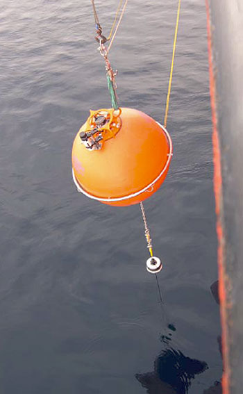
Figure 10. Top sphere deployment.
Once all the instruments and wire were in the water, the last piece of the mooring to be deployed was the 64” Syntactic sphere with a ULS and an acoustic transponder mounted to the top. A release hook was secured to the top bail of the sphere using a ‘Lift-All’ sling then attached to the ship’s crane (Figure 10).
The crane then lifted the sphere outboard of the A-Frame and the mooring was attached to the 1 m shot of Trawler Chain. The crane took the load from the vertical chain stopper so it could be removed. The top sphere was held at the surface of the water, but before being released, an acoustic range was conducted on one of the releases. About a minute after releasing the top sphere, the mooring settled at the bottom, and more ranging was conducted.
The difference between ranges gave the depth of the top sphere below the surface. The release was disabled, and each redeployment mooring operation was completed in about 5-6 hours.
11. Conclusions
Conventional deep ocean, bottom-tethered and instrumented moorings utilizing wire-rope and glass flotation technology can be routinely deployed and recovered from icebreakers in the central Arctic ice pack.
In ice-covered regions, deployments must be conducted anchor-first. To account for the added tension and ensure a responsible safety factor, heavier wire rope and hardware must be incorporated into the mooring design. Winch and windlass (or capstan) procedures are both acceptable methods of conducting the deployment. An accurate acoustic survey to determine the exact location of the mooring, adequate ice conditions, and skilled ship maneuvering are all essential requirements for a successful mooring recovery. Windlass (or capstan) procedures could be used for the recovery, but a traction winch is recommended. Backup buoyancy at the bottom of the mooring is advised for backup recovery should intermediate lengths of the mooring system get tangled under ice floes.
Acknowledgments
On behalf of all of the scientists from WHOI who participated on the JWACS/BGEP cruises on the CCGS Louis S. St. Laurent in August 2003 and August 2004, we would like to extend our sincere appreciation to all the Captains, officers, and crews and to the Canadian Coast Guard organization for the successful fulfillment of the objectives of our scientific field program in both years. We recognize that the knowledge and experience of the ship’s leaders was critical to the success of our field program, and would like to express our gratitude for the hard work, dedication, and professionalism that was demonstrated by all members during the cruises to the most inaccessible region of the Arctic Ocean. It has been a privilege and a pleasure working from the Canadian Coast Guard icebreaker, and we look forward to the opportunity to continue this cooperation in the future. Specifically for the 2004 expedition, we would like to thank Captain Andrew McNeill for his excellent leadership and ship handling skills, and Boatswain Blaine Blinkhorn and his deck crew for their expertise during the mooring operations.
Furthermore, we would like to thank IOS and JAMSTEC scientists for allowing us to collaborate and participate on the JWACS cruises, particularly Eddy Carmack (IOS), Fiona McLaughlin (IOS), Koji Shimada (JAMSTEC), and Motoyo Itoh (JAMSTEC). Special gratitude goes to Sarah Zimmermann (IOS) for her outstanding management as chief scientist on the 2004 expedition. Furthermore, we acknowledge the professional assistance that we obtained from Doug Sieberg (IOS) and Andrew Hamilton (IOS) during the field operations.
The BGFE project was funded by the NSF Office of Polar Programs ARCSS Program grant number OPP-0230184, including support for the first year of the field program (including deployment and recovery of the moorings). Any opinions, findings, and conclusions or recommendations expressed in this material are those of the authors and do not necessarily reflect the views of the National Science Foundation. Support to redeploy and recover the moorings for a second year was provided by the WHOI Ocean and Climate Change Institute.
References
Aagaard, K., C. Darnell, and F. Karig, 1978. Measurements with moored instruments in ice-covered waters, Deep-Sea Research, Vol. 25, pp. 127-128.
2003 Deployment Procedure
Cruise - Beaufort Gyre Freshwater Experiment Deployment Operations and Technology in 2003
by W. Ostrom, J. Kemp, R. Krishfield, and A. Proshutinsky
Woods Hole Oceanographic Institution
Technical Report WHOI-2004-1
Click here for print-friendly PDF version.
Table of Contents
TABLE OF CONTENTS
LIST OF FIGURES
LIST OF TABLES
ABSTRACT
1. INTRODUCTION
2. OBSERVATIONAL PROGRAM
3. MOORING DESIGN
4. DEPLOYMENT PROCEDURE
5. MOORED PROFILER
6. UPWARD LOOKING SONAR
7. BOTTOM PRESSURE RECORDER
8. SURFACE – TETHERED DRIFTERS
ACKNOWLEDGMENTS
REFFERENCES
List of Figures
Figure 1. Winter salinity, dynamic heights and geostrophic circulation in the Beaufort Gyre
Figure 2. 1979 –1997 winter and summer average sea level pressure and IABP buoy drifts
Figure 3. Results of numerical barotropic model in an ideal basin
Figure 4. BGFE mooring locations and simulated drift of BGFE ice beacons after one year
Figure 5. CCGS Louis S. St. Laurent
Figure 6. Joint Western Area Climate Study (JWACS) 2003 cruise track
Figure 7. Schematic of BGFE mooring
Figure 8. Gifford deck block
Figure 9. Fair lead block and stopper line
Figure10. Wire fair lead thru deck block to windlass capstan
Figure 11. Wire fairlead windlass capstan to tension cart
Figure 12. BGFE mooring anchor, SeaCat recorders and dual release package
Figure 13. Brailer release hook and Lift All sling
Figure 14. Sling detail: sphere deployment
Figure 15. McLane Moored Profiler
Figure 16. Mean profiles of T, S, and density at mooring locations from winter and summer
Figure 17. Upward looking sonar
Figure 18. Bottom pressure recorder
Figure 19. METOCEAN ice beacon
Figure 20. BGFE ice beacon deployed from CCGS Louis S. St. Laurent in summer 2003
List of Tables
Table 1. BGFE 2003 deployments during JWACS 2003
Table 2. Expected versus observed depths at BGFE mooring sites
Table 3. MMP deployment parameters
Table 4. Upward looking sonar deployment configurations
Table 5. Initialization of bottom pressure recorders
Table 6. Ice beacons data conversion equations
Table 7. Sample ice beacon Argos-processed data
Abstract
The Beaufort Gyre Freshwater Experiment (BGFE) observational program was designed to measure the freshwater content of the upper ocean and sea ice in the Beaufort Gyre of the Arctic Ocean using bottom-tethered moorings, drifting buoys, and hydrographic stations. The mooring program required the development of a safe and efficient deployment method by which the subsurface system could be deployed in waters surrounded by sea ice. This report documents the mooring procedure used to deploy the three BGFE moorings from the CCGS Louis S. St-Laurent, during the Joint Western Arctic Climate Study – 2003 (August 6 – September 7). The technical details of the instrumentation attached to each mooring and the specific deployment parameters are described. Specifics pertaining to the deployment of four surface-tethered drifters in the ice are also documented.
1. Introduction
The major goal of the Beaufort Gyre Freshwater Experiment (BGFE) is to investigate basin-scale mechanisms regulating freshwater content in the Arctic Ocean and particularly in the Beaufort Gyre (BG). Specifically, the variability of different components of the BG fresh water (ocean and sea ice) system will be determined, and the partial concentrations of fresh water of different origin (rivers, Pacific Ocean, precipitation, ice/snow melt, etc) will be assessed. In conjunction with historical data and model studies, an observational program was established in August 2003 to measure freshwater content (in sea ice and in the ocean) and freshwater fluxes in the BG using moorings, drifting buoys, and remote sensing. The observed freshwater content variability in the BG, which acts to integrate the complex contributions from different factors, is expected to be the primary indicator of the ocean's response to climate change.
In particular: (1) links will be identified among accumulation and release of fresh water in the BG and atmospheric, hydrologic, cryospheric and oceanic processes, (2) the regional and temporal variability of relevant processes will be quantified in terms of freshwater fluxes, and (3) the relative importance of each factor that influences freshwater content and flux change under global warming conditions will be determined. The major hypothesis of the project is that the BG accumulates a significant amount of fresh water from different sources under anticyclonic (clockwise) wind forcing, and then releases this fresh water when this forcing weakens or changes direction to a cyclonic (counterclockwise) rotation (Figures 1-3). This accumulation and release mechanism could be responsible for the observed salinity anomalies in the North Atlantic and for a decadal scale variability of the Arctic system as the BG may both filter annual river inputs and pulse freshwater outflows (Proshutinsky et al., 2003).
Support for the BGFE was provided to the principal investigator, Dr. Andrey Proshutinsky, WHOI, by the ARCSS program of the National Science Foundation. However, the project includes collaboration with other US (data sharing), Canadian (hydrographic program), UK (remote sensing) and Russian (historical data analysis) scientists. In cooperation with Institute of Ocean Sciences (IOS), Canada and Japan Marine Science and Technology Center (JAMSTEC), the Canadian Coast Guard Icebreaker Louis St. Laurent (LSL) was utilized during the Joint Western Arctic Climate Study (JWACS) cruise for the field operations in 2003. The first recovery operations are scheduled onboard the US Coast Guard Icebreaker Healy in 2004. We envision a long-term observational program in the BG to monitor changes in hydrography, ocean circulation, and ice thickness as a contribution to the anticipated NSF SEARCH program.

2.Observational program
The major objective of the observational program is to determine freshwater content and freshwater fluxes in the BG during a complete seasonal cycle. Direct measurements from the northern and western regions of the BG regions are few due to usually heavy ice conditions so modern, high-resolution data are needed to fill large spaces in the historical record. As a result, we initiated a program to acquire time series measurements of temperature, salinity, currents, geochemical tracers, sea ice draft, and sea level in the BG using moorings, drifting buoys, shipboard, and remote sensing measurements. The moorings and buoys are designed to precisely measure the variations of the vertical distribution of freshwater content and sea ice draft at representative locations (Figure 4). The hydrographic sections are to examine the variation by radius from the center of the BG. The remote sensing program will characterize the variability of the sea ice thickness (SIT) and sea surface height (SSH) horizontal structure.
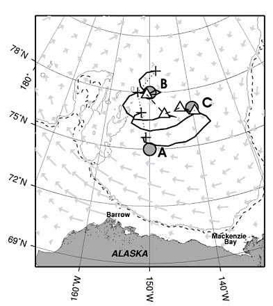
Figure 4. BGFE mooring locations (shaded circles) and simulated drift of BGFE ice beacons (triangles indicate deployment location) after one year (crosses) based on IABP monthly mean ice drift velocities (shaded arrows).
In order to keep costs manageable, the BG circulation system is assumed quasi-symmetrical and only three moorings are currently deployed for our research. Historical hydrographic and ice drift data suggest that the mean center of the BG is located near 78°N, 150°W. On the other hand, I. Rigor determined the centers for different years from IABP drift velocity grids, indicating that the Beaufort Gyre may be located farther south during positive Arctic Oscillation (AO) years. A recent surface salinity section by K. Shimada also indicates the possibility that the BG is located around 75°N. The BGFE moorings are distributed to account for both possibilities. Collaboration with other researchers will allow us to use their observations (North Pole Observatory, Bering Strait, Northern Chukchi Sea, Beaufort Sea) and to analyze their data in conjunction with our investigation.
Both icebreakers and air-supported ice camps were considered as platforms for performing the field deployment and recovery operations, and it was determined that icebreaker operations would be more practical, cost-effective, and safe. Therefore, arrangements were made to deploy our observation system in 2003 from the Canadian Coast Guard Ship Louis S. St. Laurent (Figure 5) on a Joint Western Arctic Climate Study (JWACS) cruise (Chief Scientist: Bon van Hardenberg, IOS) that departed from Kugluktuk, Canada on August 8, and returned on September 5 (Figure 6). Three WHOI scientists were responsible for installing the mooring systems and buoys with help from IOS technicians and Coast Guard personnel: Andrey Proshutinsky, principal investigator, coordinated the effort and conducted ancillary observations, Willie Ostrom lead the deployment operation, and Rick Krishfield prepared the instrumentation and assisted the deployment. More specific information on the cruise (including updates) is included on the BGFE website (https://www2.whoi.edu/site/beaufortgyre/).
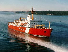
Figure 5. Canadian Coast Guard Ship Louis S. St. Laurent
In addition to the mooring and buoy deployments, shipboard hydrographic data and water sampling were carried out at 39 sites on the JWACS 2003 cruise, and about the same number will be taken in 2004. The scientific objectives of this program include: (1) identification of water mass characteristics, using multiple hydrographic tracers, and computation of freshwater content from different sources; (2) comparison of observed characteristics with historical data from the region; and (3) separation of the components of halocline water according to their origin. Temperature, salinity, oxygen, and nutrients, CFCs, carbon tetrachloride, total alkalinity, dissolved inorganic carbon, Tritium/3He and d18O will be measured. E. Carmack, R. MacDonald and F. McLaughlin from IOS, Canada are responsible for this program. Furthermore, XCTD data along the cruise data were also acquired during JWACS 2003 by K. Shimada, JAMSTEC.

Table 1. BGFE 2003 Deployments During JWACS 2003
(All times = GMT – 6 hours)
Mooring A:
Deployed August 14, 2003 07:51 75° 00.53’ N 150° 00.12’ W begin
12:20 75° 00.39’ N 149° 58.752’ W dropped
CTD depth = 3820 m; Sound speed = 1480.1 m/s
Ship sounder = 3775 m; Sounder II = 3790 m
Release depth after deployment = 3819 m
Mooring B:
Deployed August 23, 2003 17:37 78° 01.254’ N 149° 51.148’ W begin
22:05 78° 01.491’ N 149° 49.378’ W dropped
CTD depth = 3823 m; Sound speed = 1480.4 m/s
Ship sounder = 3770 m
Release depth after deployment = 3824 m
Landing minus drop distance = 48 m (3814-3766 m, transducer at 10 m)
Mooring C:
Deployed August 26, 2003 15:03 76° 59.49’ N 140° 01.54’ W begin
19:03 76° 59.254’ N 139° 54.229’W dropped
CTD depth = 3726 m;
Release depth after deployment = 3733 m
Landing minus drop distance = 80 m (3723-3643 m, transducer at 10 m)
Buoy 1:
ARGOS ID = 40298 Ice thickness = 3 m
Deployed August 23, 2003 09:35 77° 58.5’ N 150° 44.6’ W on ice
11:00 77° 58.6’ N 150° 42.6’ W off ice
Buoy 2:
ARGOS ID = 40300 Ice thickness = 2 m
Deployed August 25, 2003 11:30 76° 51.5’ N 146° 41.7’ W ship in position
12:30 76° 51.568’ N 146° 39.601’W buoy deployed
Buoy 3:
ARGOS ID = 40297 Ice thickness = 1.9 m
Deployed August 26, 2003 07:00 77° 06.5’ N 142° 47.5’ W site selected
07:51 77° 06.4’ N 142° 47.4’ W off ice
Buoy 4:
ARGOS ID = 40299 Ice thickness = 2.4 m
Deployed August 26, 2003 20:30 76° 50.04’ N 139° 29.93’ W ship in position
22:00 76° 49.9’ N 139° 29.3’ W off ice
3. Mooring design
Moorings provide time series of T, S, currents, sea ice draft, and bottom pressure (sea surface heights). A robust, economical system is utilized to obtain high-accuracy, long-term vertical profiles of ocean temperature, salinity and velocity in the BG (Figure 7). Conventional mooring systems containing a McLane Moored Profiler (MMP) are used to sample currents and hydrographic data from 50 to 2050 m with a 54 hours time interval. In addition, an ASL Environmental Sciences 420kHz upward-looking sonar (ULS) provides information about sea ice draft, and a high accuracy bottom pressure recorder (BPR) measures sea level height variability and near bottom T and S. Each mooring consists of a surface flotation package housing an ULS, a mooring cable containing the MMP (5/16” jacketed wire rope, breaking strength 9800 lb.), dual acoustic releases and tether to BPR attached to the anchor. 1/2” Trawler chain (breaking strength > 9800 lb.) is used between the releases and anchor.
The surface floatation package is a 64” syntactic foam sphere with mounting for the ULS and acoustic transponder. It is located at 46 m so that the upper limit of the profiling instrument may be at 50 m. The profiler will travel along a single 2000 m (stretched length) segment of plastic jacketed wire rope with bumper stops at end. Beneath the lower end of the profiler mooring segment, other shots of wire rope and glass floatation balls provide the strength and buoyancy to maintain the 3800 m long mooring system vertically. Dual Edgetech acoustic releases attach the positively buoyant mooring system to the 3800 lb anchor tethering the system to the bottom. A BPR is mounted on the anchor using a specially designed bracket.
In order to ensure that the uppermost MMP bumper is located as close as possible to 50m, adjustment cables shots will be employed to correct the mooring length to the exact depth during deployment. Upon arriving on station to deploy the moorings, a CTD is performed to adjust the depths soundings for the speed of sound. The expected error of the depth estimate can be as large as +/- 20 m. The mooring itself is provided with a lot of buoyancy and should be very rigid. According to a dynamical model of the vertical mooring variation, a 50 cm/s current at 50 m superimposed on a 5 cm/s background depresses the surface buoyancy float only 2 m on the 3800 m long mooring. Assuming a relatively flat ocean bottom, adjustment lengths will be used to adjust the mooring length to within a meter, so the final vertical placement of the uppermost float is expected to fall within +/-10 m of 46 m below the surface.

The expected depths at the mooring sites and surrounding grid cells from the ETOPO5, ETOPO2, and IBCAO datasets are reasonably close to the depths determined during JWACS 2003 from CTD casts:
Table 2. Expected versus observed depths at BGFE mooring sites
ETOPO5 ETOPO2 IBCAO JWACS
A 75N, 150 W: 3835 3838 3840 3813 3813 3814 3814 3816 3817
3829 3831 3833 3818 3819 3819 3828 3827 3826 3820
3824 3826 3828 3823 3823 3824 3830 3829 3828
B 78N, 150W: 3684 3718 3749 3725 3725 3725 3726 3726 3726
3678 3710 3742 3726 3726 3726 3726 3726 3726 3823
3697 3726 3754 3726 3726 3726 3726 3726 3726
C 77N, 140W: 3684 3683 3681 3703 3703 3703 3704 3704 3704
3691 3690 3689 3704 3705 3705 3708 3709 3709 3726
3698 3697 3696 3708 3709 3709 3700 3703 3706
The length of the BGFE moorings that were deployed were: site A = 3750 m, site B = 3775 m, site C = 3662 m. The difference from the bottom gives the approximate depth of the top sphere.
The actual mooring positions and measured water depths for all BGFE mooring are listed in Table 1.
4. Deployment Procedure
The three BGFE moorings were deployed in 2003 using an anchor first technique developed by the WHOI - Mooring Operations, Engineering and Field Support Group. The methods of the deployment and recovery of deep-ocean moorings through sea-ice from icebreaker have been used by members of WHOI on the Healy in the Labrador Sea trials, during the Shelf-Basin Interactions Program (SBI), and were employed in the Ross Sea, Antarctica to recover sediment trap moorings during JGOFS.
The standard method for deployment of a mooring of this type would normally be anchor last, which minimizes the tension on the mooring segments during the deployment operation. This method begins with the ship positioned down wind from the desired anchor location approximately two and half times, the overall length of the mooring. The top segment of the mooring is deployed first over the stern of the ship, the ship slowly transits towards the anchor drop site as mooring components are connected and passed over the side, and with the entire mooring towing behind the ship, the anchor is cast over the stern completing the deployment. However, this method requires a large amount of open water to stream the mooring behind the ship so is not practical in ice-covered oceans. Because of the potential for large ice flows existing in the area of the BGFE mooring sites, the following anchor first procedure was adopted.
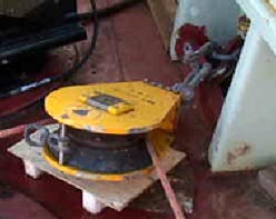
Figure 8. Gifford deck block.
Mooring operations on CCGS Louis S St. Laurent were conducted from the fore deck. The starboard A-frame was rigged with a WHOI Gifford mooring block secured to the A-frame center bale and a vertical chain stopper attached to the adjacent forward bail. A 4 meter length of ½ inch trawler chain was used for the vertical stopper. A ½ inch chain grab was shackled onto the vertical chain stopper approximately 0.5 meters from the deck. A second Gifford block (Figure 8) was secured to a custom fairlead bail welded to the main hatch combing. A 10 ft. LiftAll SN 60 sling was barrel hitched around the base of the ship’s starboard bow compressor. A 10” McKissick 5CC snatch block was hooked onto both ends of this sling (Figure 9). The position of the block allowed a 2 ton snap hook with an attached 7/8 inch Sampson stopper line when bent through the block to be in aligned with the windlass capstan.

The mooring wire fairlead ran from through the A-frame block down through the deck block and 9 times around the windlass capstan. The mooring wire exiting forward from the windlass capstan was bent around the ship’s turning fairlead and redirected aft to a Reel-O-Matic tension reel stand. Figures 10 and 11 show opposing views of the mooring wire fairlead.


The personnel utilized for the safe payout of the mooring wire required: a Boatswain, mooring operations supervisor, windlass operator, two windlass wire handlers, tension cart observer, mooring log recorder and acoustic release technician. The Boatswain’s responsibilities were to direct all shipboard deck machinery and maintain communications with the ship’s bridge. The correct construction and deployment of the mooring rested upon the mooring operations supervisor. The windlass operator and windlass wire handlers were responsible in maintaining control of the mooring wire rope warped around windlass capstan. The tension cart observer maintained constant visual inspection of the cart’s operation. The responsibilities of the mooring log recorder were to verify and document the mooring components as they were deployed. Because the mooring wire was being manually controlled over the windlass capstan, one of the two acoustic releases attached to the anchor was enabled so that the acoustic release technician could instantaneously send a release command to jettison the 3800 lb. anchor if the payout got out of control.
The mooring deployment commenced following a CTD cast to determine an accurate water depth. The ship’s position over the anchor site was maintained during the mooring operation. The mooring anchor was positioned using the starboard crane into the center of the A-frame. The duel acoustic releases were moved along side of the anchor and the release chain was bent through the 1 ¼ inch Master link shackled to the anchor. The ends of the release chain were inserted into the release armatures and the releases were armed. A 3 meter length of ½ inch chain was shackled to the top bale of the duel release tension bar. The starboard crane swung over the acoustic releases and the crane’s whip lowered hooking onto the ½ inch chain approximately .5 meters from the chain’s free end, using a. 8 ft. LiftAll SN 60 sling barrel hitched through a ½ inch chain grab. The crane whip was hauled in lifting up the chain and duel releases over the top of the anchor. The anchor was suspended off the deck, to allow any existing rotary motion in the linkage’s from the release chain and attaching hardware to unwind. The anchor was lowered transferring enough of the anchor’s weight onto the deck to stabilize the anchor. The bottom pressure recorder was inserted into its containment tube attached to the side of the anchor. A half clamp bracket was bolted to the acoustic release case closest to the pressure recorder. A Tygon tube incased length of 5/16 inch proof coil chain was shackled to the pressure recorder’s top bail. The free end of the chain was shackled to the bracket bolted to acoustic release. Figure 12 details this assembly. When the anchor is released, the recorders will be pulled from the mount by the smaller chain.

The bridge was notified that the anchor was ready to be lowered over the side. With confirmation to proceed, the crane lifted the anchor up and out board of the ship’s starboard side. The anchor was lowered until the chain grab hooked to the ½ inch chain was 1 meter from the deck. The ½ inch chain grab attached to the vertical chain stopper was hooked onto the hanging mooring chain, 0.5 meters from the deck. The crane whip lowered and its chain grab was removed. The next mooring segments to be deployed were the 30 17 inch glass balls bolted onto ½ inch chain. The glass balls were pre-connected into 8 glass balls/8 meter lengths. The crane’s boom shifted inboard and the crane’s hook and slung chain grab were hooked between the 6th and 7th glass ball. It was found that this number of glass balls was the maximum manageable number of glass balls that could be lifted inside the A-frame at one time. The crane whip hauled in lifting the glass ball string off the deck and taking on the hanging mooring tension, which allowed the vertical chain stopper to go slack and be removed. The crane boomed down to allow the glass balls to clear the side of the ship. The glass balls were lowered until again the crane whip’s chain grab was 1 meter from the deck. The vertical chain stopper was hooked below the crane whip’s chain grab. The crane whip lowered transferring the mooring tension to the vertical chain stopper. This procedure was repeated until all 30 glass ball were hanging from the vertical chain stopper.
The first wire shot to be shacked to the free ½ inch chain end of the deployed glass balls was pulled from the tension cart forward around the ship’s turning block, up over the top of the windlass capstan and bent around 9 times. The wire was then revved thru the deck and A-frame fairlead blocks and down to the hanging glass balls. The wire rope termination was shackled to the free end of the ½ inch chain. The windlass was hauled in drawing in the wire rope taking the mooring tension away from the vertical chain stopper. The vertical chain stopper’s ½ inch chain grab was removed and the A-frame shifted out board as the windlass paid out, allowing the wire rope to be lowered over the side. The windlass wire handler positioned out side of the wire rope bite which ran from the turning block to the tension cart, maintained a consistent grip on the wire so that the wire rope would not slip around the capstan barrel, in order to prevent chaffing on the wire rope’s polyethylene jacket. The vigilance of the windlass wire rope handler in laying the wire rope onto the capstan head correctly with ample back tension was critical to the safe lowering of the heavily loaded mooring components. The tension cart observer periodical adjusted the cart’s hydraulic valve to maintain an adequate level of additional resistance to the wire rope running to the windlass wire handler and visually checked that the storage wire rope reel was not moving out of alignment. The payout speed of a wire shot was at the maximum speed of the windlass was approximately 25 meters per minute.
When the last wire rope lay became exposed on the storage reel, the windlass speed was reduced and a second wire handler was positioned in front of the tension cart to manually monitor the wire rope as its bitter end came off the reel. Once the bottom end of the wire rope had been removed from the storage reel, the second wire handler firmly gripped the wire just ahead of the wire rope termination and assisted in applying additional back tension pulling against the windlass capstan. A 5/8 inch shackle and 5/8 inch pear ring were connected to the wire rope termination. The windlass capstan slowly paid out and second wire rope handler holding onto the hardware moved around the turning block up to the capstan wire handler. A snap hook attached to a 7/8 inch diameter Sampson stopper line was connected onto the 5/8 inch pear ring. The Sampson line was drawn tight and secured across the ship’s bits. The capstan paid out allowing the stopper line to take on the load held by the capstan wire handler. With mooring stopped off, the empty storage reel was removed and the next wire rope reel installed onto the tension cart. The wire rope termination coming off the top of the storage reel was pulled up around the turning block and shackled to the stopped off termination. The windlass and second wire handlers assumed their positions out side the bite and held back on the mooring wire. The capstan hauled in slightly with the wire handlers taking up the loose slack, the stopper line was removed. A WHOI Velcro canvas cover was wrapped around the hardware joining the two wire shots. The capstan slowly paid out as the two wire handlers applied back tension. While the termination bundle wound around the capstan barrel, the wire helix tended to snap towards the center of the barrel. The wire handlers had to grip the wire very tightly during this phase of the payout in order to prevent the wire rope from getting fouled on the capstan. The canvas wrap shrouding the terminations was removed once it had passed through the two fairlead blocks and reached out board of the A-frame approximately 2 meters from the deck. A 3 ton snap hook shackled to the vertical chain stopper 1 meter from the deck was hooked onto the 5/8 inch pear ring and the windlass paid out allowing the upper termination to be disconnected. A 4 glass ball segment was positioned to the vertical chain stopper and shackled onto the stopped off pear ring. The loose wire rope termination was reattached to the free end of the glass ball chain and the capstan hauled in lifting the glass balls off the deck. Once the tension was off the vertical chain stopper, the snap hook was removed and payout commenced. The McLane moored profiler, MMP was deployed in a similar fashion. The end of the last wire shot was paid out using a 7/8 inch diameter Sampson winch line, where it was stopped off using the vertical chain stopper.
The 64 inch syntactic sphere at the top of the mooring was pre-positioned aft along side the A-frame. A 1 meter ½ inch trawler chain and a 3 ton Miller swivel were shackled onto the sphere’s bottom bail. This assembly had a ¼ inch manila line tied to the 5/8 inch pear ring joining the swivel and the ½ inch chain. The line’s bitter end was tied to the sphere’s equator ring with a slip bowline so that when the sphere was suspended in the A-frame, the line could be easily reached. A 10 ft. LiftAll SN 60 sling was barrel hitched through one of the sphere’s lifting bail. The release hook used to deploy the sphere was a Brailer release hook with a 6 ft. LiftAll SN 60 sling shackled with a 5/8 inch shackle to one of the side bail of the hook. This shackle was assembled so that the thumbscrew would protrude away from the release pin. Figure 13 illustrates this assembly.
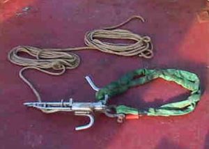
Figure 13. Brailer release hook and Lift All sling.
Once the 1995 meter length of wire rope had been paid out and stopped off onto the vertical chain stopper, the ship’s starboard crane swung over the sphere. The 10 ft. sling was barrel hitched onto the crane whip hook .The A-frame shifted inboard so that the hanging wire rope was approximately 0.5 meter away from the side of the ship. The Sampson winch line was passed out board of the A-frame and shackled to the Brailer hook. The sling secured to the Brailer hook was passed through an inboard sphere bail and secured to its release pin. The Brailer release line was passed out board and forward around the A-frame base brings the line inside the A-frame. The sphere was lifted and swung out board of the A-frame.
The ¼ inch manila tag line slip knot tied to the sphere was untied so that the free end of the ½ inch chain and attached swivel could be shackled to the stopped off mooring wire. The crane whip hauled in lifting the sphere, taking the mooring tension from the vertical chain stopper. This stopper was removed. The crane slowly lowered the sphere transferring the hold on the mooring to the Brailer hook and Sampson winch line revved around the windlass. Figure 14 shows the crane whip sling and Brailer hook orientation during this transfer.
The 10 ft. sling was removed and the crane swung clear of the A-frame. The A-frame shifted out board as the windlass paid out lowering the sphere. The Brailer hook release line was carefully tended so that the line was slack during this phase of the operation. Once half the sphere’s diameter had been submerged, payout was stopped and the acoustic releases were ranged upon to check the overall length of the mooring relative to the water depth. Upon completion of this test the Brailer hook release line was tied off to an A-frame cleat and the windlass lowered the sphere transferring the mooring tension to the release line, causing the hook to open casting off the mooring. Once the mooring anchor had settled on the sea bottom, the acoustic releases were ranged upon to determine the position of the mooring.

5. Moored Profiler
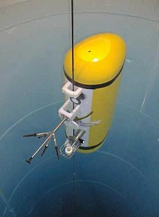
Figure 15. McLane Moored Profiler
The McLane Moored Profiler (MMP) is an autonomous, instrumented platform on a conventional mooring tether, which repeatedly traverses that line based on a user defined operation program, acquiring in situ profiles of temperature, salinity and velocity (Morrison et al., 2000). Figure 15 shows the MMP on a mooring wire in a test tank.
The maximum depth rating is 6000 m, and design endurance is over one million meters per deployment. The system software gives the operator great flexibility in defining the sampling schedule, allowing profiles to be interspersed with extended measurements at fixed levels. The along-cable speed of the MMP is approximately 25 cm/s. This speed is determined by the need to minimize energy expenditure to increase the deployment duration. Accurate ballasting of the instrument for the seawater characteristics during the deployment is necessary for proper operation. Using the GDEM interpolations from the EWG summer and winter atlas data, representative profiles for the BGFE mooring locations were selected (Figure 16). The differences between the different seasons and locations is small, so the instruments on different moorings can be ballasted from the same values. The neutral water column values were estimated from the average of the upper (50m) and lower values (2050m) from the representative profiles: neutral depth = 1000 m, neutral temperature = -1.0 °C, neutral salinity = 32.9, and neutral density = 1031.2 kg/m3.
The CTD and current measurement instruments presently employed on the MMP are products of Falmouth Scientific, Inc. The MMPs used for the BGFE are newly manufactured instruments that have been tank tested and dock tested, with factory calibrated CTDs and ACMs. A problem with ACM pressure compensating fluid leaks was detected during the dock tests and repaired. In addition, the heading bias of the ACM compass resulting from the magnetic field of the battery packs was recorded for each MMP by performing spin tests (112 = 18.3°, 113 = 25.4°, 114 = 23.23°). The biases must be subtracted from the measured angles to provide true directions. Eccentricity of the ACM measurement is also a concern, and while measurements were conducted in the lab, post-cruise processing of the data will provide better corrections.

The parameters that were used to program the MMPs for the BGFE experiment are selected to ensure a minimum duration of 400 days (800,000 km), and to enable the M2, S2, O1, and K1 tidal constituents to be quantified. Table 3 lists these parameters.
Table 3. MMP deployment parameters
BGFE-A (114) Z| Scheduled start = 08/15/2003 12:00:00
Estimated Profile 1 start time: 08/15/2003 18:00:00
BGFE-B (113) Z| Scheduled start = 08/24/2003 12:00:00
Estimated Profile 1 start time: 08/24/2003 18:00:00
BGFE-C (112) Z| Scheduled start = 08/27/2003 04:00:00
Estimated Profile 1 start time: 08/27/2003 12:00:00
Schedule I| Profile start interval = 000 06:00:00 [DDD HH:MM:SS]
R| Reference date/time = 08/01/2003 00:00:00
B| Burst Interval = 002 06:00:00 [DDD HH:MM:SS]
N| Profiles per burst = 2
P| Paired profiles Disabled
F| Profiles / file set = 10
Stops S| Shallow pressure = 30.0 [dbar] D| Deep pressure = 2000.0 [dbar] H| Shallow error = 40.0 [dbar] E| Deep error = 200.0 [dbar] T| Profile time limit = 02:50:00 [HH:MM:SS] C| Stop check interval = 15 [sec]
6. Upward Looking Sonar
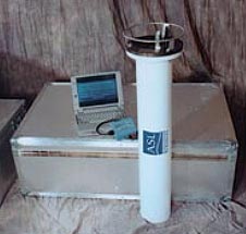
Figure 17. Upward looking sonar
Upward looking sonar IPS4, (Figure 17) manufactured by ASL Environmental Sciences, are mounted in the uppermost flotation to sample the ice draft with a precision of +/- 0.05 m in acoustic range, or typically +/- 0.3m after conversion to ice thickness. Originally designed at IOS (Melling et al., 1995), the systems determine the return travel time of a 420 kHz acoustic pulse (1.8° beam at –3 dB) reflected from sea ice, or the surface. The “footprint” of the measurement is less than 0.5 m at 30 m operating depths. A pressure sensor (Paroscientific Digiquartz) is incorporated to measure the sea level changes due to winds and tides, and the vertical changes in the mooring length due to current drag.
The battery pack provides approximately 80 Ah, and the storage capacity is 64 Mbytes. In addition to the travel time, the maximum amplitude and the persistence (duration) of the selected echo may be recorded. To reduce memory requirements, pressure and tilt are recorded less frequently than each travel time (every 20 records), and burst measurements (for ice free periods) less frequently (every 510 records). Software provided by ASL, IpsLink (Version 2.00.04) allows different deployment schemes to be prepared and power and data storage requirements assessed. Parameters selected for the BGFE deployment extend the battery life to a full year using a 2 second ping rate, and leaves sufficient memory to record the amplitude and persistence. Table 4 lists these parameters.
Table 4. Upward looking sonar deployment configurations
BGFE-A Unit '1038' deployed 2003-08-13 02:23:33
Setting deployment name to 'bgfe03Ax' and number of phases to 1 ... PASSED
Setting phase 1 start date set to: 03/08/14/00 ... PASSED
BGFE-B Unit '1037' deployed 2003-08-21 15:42:23
Setting deployment name to 'bgfe03Bx' and number of phases to 1 ... PASSED
Setting phase 1 start date set to: 03/08/22/00 ... PASSED
BGFE-C Unit '1036' deployed 2003-08-25 19:44:48
Setting deployment name to 'bgfe03Cx' and number of phases to 1 ... PASSED
Setting phase 1 start date set to: 03/08/26/00 ... PASSED
Setting phase 1 Ping Interval to 2 ... PASSED
Setting phase 1 Ping Length to 68 ... PASSED
Setting phase 1 Lockout to 10 ... PASSED
Setting phase 1 Maximum Range to 90 ... PASSED
Setting phase 1 Pressure Interval to 20 ... PASSED
Setting phase 1 Burst Interval to 510 ... PASSED
Setting phase 1 Burst Count to 1 ... PASSED
Setting phase 1 Record Persistence to n ... PASSED
Setting phase 1 Record Amplitude to y ... PASSED
Setting phase 1 Minimum Persistence to 8 ... PASSED
Setting phase 1 Start Amplitude to 200 ... PASSED
Setting phase 1 Stop Amplitude to 150 ... PASSED
Looking for confirm phase line from FIRMWARE ... PASSED
Reading phase confirmation data from FIRMWARE ... PASSED
Confirming phase 1 ... PASSED
Confirm deployment set to 'y' ... PASSED
Erasing Solid State Memory ... deployment started
Ice thickness is computed from the difference between the instrument depth and the range to the underside of the sea ice. Depth is determined from the hydrostatic equation, using the pressure measurements adjusted for atmospheric pressure (which must be obtained elsewhere). The range is corrected for instrument tilt and speed of sound differences (which may be estimated from the uppermost MMP data and open water events).
7. Bottom Pressure Recorder
Precise bottom pressure measurements will be made using Sea-Bird Electronics SBE-16plus temperature and salinity recorders, (Figure 18) with precision Paroscientific Digiquartz (6000 psia) pressure sensors. The resolution of the pressure measurement depends on the sensitivity of the sensor and the resolution of the counter. Integrating the pressure measurements increases the resolution of the pressure measurement, although this may be limited somewhat by sensor drift, recorder time base drift, and background noise.

Calibration was performed prior to use to observe the error of the measurement, due primarily to the pressure sensor drift and the time base drift of the recorder. Furthermore, the engineer at SeaBird Electronics indicated that there is a startup transient during the warmup of the 6000 psia Digiquartz sensor. Power considerations do not allow for the measurement to start after the warmup, so the measurement occurs with some transient bias still applied. The error that results is only as large as the variability of the transient bias, which is probably small, but unknown. In order to quantify the combination of all of these uncertainties, each pressure sensor was exercised for a number of days using a dead-weight tester at the approximate pressure that it will be deployed (3800 m), and sensor drift was compared with measurements by a standard.
For the transducer applicable to our application, a measurement integration of 70 seconds should resolve better than 1 mm. At a 25 minute sample rate, the lithium batteries will provide sufficient power for over a full year (410 days) of measurements. Table 5. lists the bottom pressure recorders battery voltage,sample rate and state up times.
Table 5. Initialization of bottom pressure recorders
BGFE-A SBE 16plus V 1.6a SERIAL NO. 4413 10 Aug 2003 20:48:31
vbatt = 10.7, vlith = 8.7, ioper = 52.1 ma,
waiting to start at 12 Aug 2003 00:00:00
BGFE-B SBE 16plus V 1.6a SERIAL NO. 4414 23 Aug 2003 18:26:30
vbatt = 10.7, vlith = 8.8, ioper = 53.1 ma,
waiting to start at 23 Aug 2003 21:00:00
BGFE-C SBE 16plus V 1.6a SERIAL NO. 4415 25 Aug 2003 20:29:48
vbatt = 10.7, vlith = 9.0, ioper = 53.3 ma,
waiting to start at 27 Aug 2003 23:00:00
sample interval = 1500 seconds, number of measurements per sample = 1
Paros integration time = 70.0 seconds
samples = 0, free = 524288
no pump, delay before sampling = 0.0 seconds
transmit real-time = no
battery cutoff = 7.5 volts
pressure sensor = quartz with temp comp, range = 6000.0
SBE 38 = no, SBE 50 = no, Gas Tension Device = no
Ext Volt 0 = no, Ext Volt 1 = no, Ext Volt 2 = no, Ext Volt 3 = no
echo commands = yes
output format = raw HEX
serial sync mode disabled
In order to ensure that the measured pressures do not include any mechanical movement due to the mooring, the BPRs are mounted on the anchors (Figure 12). The SeaCats are tethered to the releases, using chain and mounted and tie-wrapped in an aluminum tube on the anchor for deployment. Upon release of the mooring system, the tether will retrieve the BPRs from the anchor.
8. Surface-tethered drifters
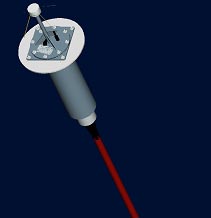
Figure 19. METOCEAN ice-beacon
Observations and numerical simulations indicate that the freshwater content variations in the BG due to Ekman forcing should extend far below the surface mixed layer (deeper than 1000~m). Timeseries integrations of the vertical profile data from the moorings will be used to precisely quantify the seasonal changes in the upper ocean freshwater content in the upper 50-2050 m. A gap in the measurements exists above 50 m below the surface, where the mooring systems terminate in order to avoid interactions with the submerged portions of ice islands or deep pressure ridges. Hence, several economical ice-tethered drifters, (Figure 19) were deployed in August 2003 to provide concurrent T & S data at several discrete depths in the uppermost 40 m.
METOCEAN expendable ice beacons suspend 3 SeaBird MicroCats at 15, 25 and 40 m depths (the deepest MicroCat also has a pressure sensor to determine depth), interrogate each sensor twice per day, and broadcast the data via Argos, which also provides each drifter’s location. These ice drift timeseries are immediately made available to the IABP and GTS. The temperature and salinity data are updated daily on the BGFE website.
During the JWACS 2003 cruise, 4 ice beacons were deployed in a radial section through the BG upstream of the moorings, so that the ice drift will transport the buoys past the moorings (Figure 4). Due to relatively thin ice conditions during August, it was difficult to find multiyear icefloes thicker than 2 m. Large icefloes were selected during the cruise from RADARSAT maps and ice reconnaissance flights on helicopter. The actual buoy deployment site was selected after auguring several small holes at different locations, on other sides of consolidated ridges.

Typically, the ice thickness was about 1.5 m, with the bottom half saturated with water. Somewhat thicker ice was generally found in areas surrounded by ridges.
Each ice beacon was completed assembled on the ship, operational, and organized in a pallet box prior to arriving on site. Two sled loads were required during each deployment to transfer the auger and ice beacon to the selected site several hundred meters from the ship. A 10” hole was augured through the multiyear ice floe, and the sensor string (with 30 lb weight) was lowered through the ice by hand. Then a wooden platform was assembled around the buoy to distribute the thermal effect of the ice beacon, and shield the upper ice. Finally, snow was piled on the wood to provide further insulation. The ice beacons have power to obtain measurements for over 1 year, but have no flotation so will eventually melt through the ice and sink. Figure 20 shows a deployed ice beacon.
The ice beacon data are acquired and decoded by Service Argos, according to the manufacturer’s equations listed in table 6.
Table 6. Ice beacon data conversion equations
These data and the platform locations derived by Argos are copied to a computer at WHOI and emailed to the PIs on a daily basis, and bi-weekly archives are provided on CD. Table 7 is a sample of the Argos data for an ice beacon several days after deployment.
Table 7. Sample ice beacon Argos-processed data
02668 40297 31 12 K 3 2003-08-30 17:40:13 77.353 218.258 0.000 401648073
2003-08-30 17:33:37 1 58 0.00000E+0 0.33100E+3 0.17200E+2
-.14085E+1 0.22966E+1 -.13505E+1 0.23452E+1
-.12215E+1 0.24508E+1 0.43480E+2 00
2003-08-30 17:35:05 1 113 0.10000E+1 0.33300E+3 0.17200E+2
-.13600E+1 0.23104E+1 -.13520E+1 0.23457E+1
-.12045E+1 0.24507E+1 0.43502E+2 00
2003-08-30 17:36:33 1 213 0.20000E+1 0.33400E+3 0.17200E+2
-.14360E+1 0.23063E+1 -.13530E+1 0.23504E+1
-.12125E+1 0.24480E+1 0.43520E+2 00
2003-08-30 17:38:01 1 62 0.00000E+0 0.33500E+3 0.17200E+2
-.14085E+1 0.22966E+1 -.13505E+1 0.23452E+1
-.12215E+1 0.22204E+1 0.43480E+2 00
2003-08-30 17:39:29 1 117 0.10000E+1 0.33700E+3 0.17200E+2
-.13600E+1 0.23104E+1 -.13520E+1 0.23457E+1
-.12045E+1 0.24507E+1 0.43502E+2 00
2003-08-30 17:40:57 1 217 0.20000E+1 0.33800E+3 0.17200E+2
-.14360E+1 0.23063E+1 -.13530E+1 0.23504E+1
-.12125E+1 0.24480E+1 0.43520E+2 00
2003-08-30 17:42:25 1 67 0.00000E+0 0.34000E+3 0.17200E+2
-.14085E+1 0.22966E+1 -.13505E+1 0.23452E+1
-.12215E+1 0.24508E+1 0.43480E+2 00
2003-08-30 17:43:53 1 121 0.10000E+1 0.34100E+3 0.17200E+2
-.13600E+1 0.23104E+1 -.13520E+1 0.23457E+1
-.12045E+1 0.24507E+1 0.43502E+2 00
2003-08-30 17:45:21 1 222 0.20000E+1 0.34300E+3 0.17200E+2
-.14360E+1 0.23063E+1 -.13530E+1 0.23504E+1
-.12125E+1 0.24480E+1 0.43520E+2 00
2003-08-30 17:46:49 1 71 0.00000E+0 0.34400E+3 0.17200E+2
-.14085E+1 0.22966E+1 -.13505E+1 0.23452E+1
-.12215E+1 0.24508E+1 0.43480E+2 00
Acknowledgments
Captain Bryan Gibbons and the officers and crew of the CCGS Louis S. St Laurent deserve special thanks for their high level of professionalism through out the JWCAS 2003 cruise, and in particular during all the mooring operations. Even with the potential risks involved with anchor first mooring deployments, the ship’s Boson and deck crew performed all deck operations in a time efficient and safe manner. We thank chief scientist, Bon van Hardenberg (Institute of Ocean Sciences, IOS, Canada), for his support during the cruise, Doug Sieberg (IOS) for his expert assistance with the mooring acoustic survey, Humphrey Melling (IOS) for recommendations on configuring the upward looking sonar, and John Toole (WHOI) for advice on testing and preparing the MMP. We acknowledge the contributions by E. Carmack (IOS), F. MacLaughlin (IOS), K. Shimada (JAMSTEC), and M. Bergmann (DFO, Canada). The preparation of the mooring systems utilized the expertise of the WHOI Rigging shop (R. Trask, J. Reese), Mooring Operations Group (S. Murphy, J. Dunn), and Instrument Shop (Ryan Schrawder, Scott Worrilow). The Beaufort Gyre Freshwater Experiment is supported by the National Science Foundation under Grant No. OPP-0230184.
References
Melling, H., P.H. Johnston, and D.A. Riedel, “Measurements of the underside topography of sea ice by moored subsea sonar,” J. Atmos. and Oceanic Tech., 12, 589-601, 1995.
Morrison, A.T., III, J.D. Billings, and K.W. Doherty, “The McLane Moored Profiler: An Autonomous Platform for Oceanographic Measurements,” Proceedings of OCEANS 2000, MTS/IEE/OES, Vol. I, 353-358, 2000.
Proshutinsky, A., R.H. Bourke and F.A. McLaughlin, The role of the Beaufort Gyre in Arctic climate variability: Seasonal to decadal time scales, Geophys. Res. Lett., 29(23), doi:10.1029/2002GL015847, 2002.