INTRODUCTION

Packets of nonlinear internal waves (NIW) have been observed throughout the world, primarily on continental shelves. These waves are sometimes referred to casually as solitary waves, solitons, or solibores. We choose to use a more inclusive, generic name because of the uncertainty between our observations and the dynamics implied by the other terms.

These waves are generated by the interaction of the tide with topography, such as sills and continental slopes. In recent years NIW have commanded the attention of a diverse group of researchers studying: geophysical fluid dynamics, acoustics, ocean optics, sediment transport, plankton advection and vertical mixing. This conference provides an opportunity to ask a fundamental question of all disciplines: Why study nonlinear internal waves? Two answers come to mind: they are interesting, and they may be important.

Demonstrating that they are interesting is easy. They often make a striking appearance in observations, commanding attention. They invite explanation of fluid dynamicists and are probably worth studying in name of knowledge for its own sake.

As to whether they are important, the reason may depend upon the discipline answering the question, and we are eager to learn the viewpoints of others. As for physical oceanography, one of the measures for importance is: Do nonlinear internal waves contribute significantly to mixing on continental shelves?

We will discuss our observations of NIW highlighting how they relate to the issues of interest and importance.

OBSERVATIONS: Interesting?

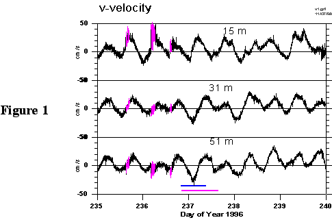
The observations presented here were obtained from a mooring in the Mid-Atlantic Bight (40.5 deg N, 70.5 degW) during the Coastal Mixing & Optics / SAS Primer experiment. Temperature and velocity time series were recorded from July through September 1996 spanning the 70 m water depth. It is instructive to look at the NIWs in the context of the oscillations at other scales that are due to other processes. For example, the 5-day time series of northward velocity shown in Figure 1 is dominated by the semidiurnal tide, which is primarily barotropic.

NIWs appear as high-frequency packets separated by about 12 hours during the first 2 days; the NIWs are nearly absent in the last 3 days. The background oceanic conditions do not change much during this time, but the NIW signal does.
 
 

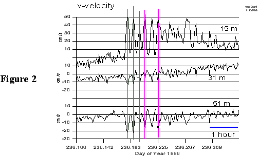
Expanding the time axis for one packet (Figure 2), we can see the packet is composed of 6 large "solitons". (Note: we use the term soliton here for convenience rather than to imply that these satisfy the precise fluid mechanical definition of soliton.) The velocity pulses are indeed significant, reaching 40 cm/s in the upper layer. The vertical structure is consistent with mode 1 behavior with a zero-crossing near 30 m depth. Each soliton has a temporal width of about 10 minutes. The corresponding temperature signal of this packet shows that the solitons are waves of depression with vertical displacements of up to 15 m.
 

Despite the regularity of the barotropic tide, the characteristics of the NIWs vary in time. To summarize this variability, statistics were compiled of all packets that were observed during a 60 day period(Figure 3). These statistics are based on certain subjective criteria in defining a signal as a soliton. There are undoubtedly many less energetic NIWs that
 
 

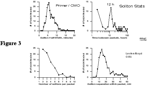
escaped our census. Packets are most often separated by about 12 hours as expected for semidiurnal generation. However, there are often gaps in this regular generation, as seen in Figure 1, and the separation between packets is often longer than 12 hours. The number of solitons in a packet also varies-most packets contain only 2 or 3, and they are not always rank ordered. The temporal width of the individual solitons was peaked around 10 minutes, with a significant number that were "wider". 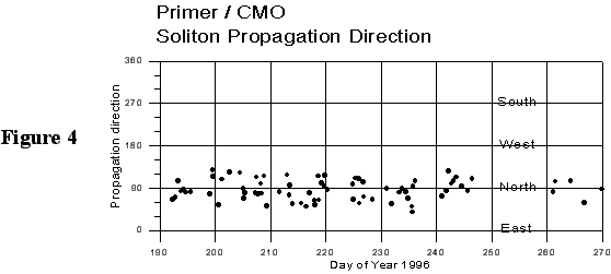No attempt has yet been made to account for the effect of the low frequency tidal flow on this estimate of width. The propagation direction (Figure 4) of the packets was determined by looking at the velocity in the upper layer. On average the waves were definitely propagating onshore (northward) perpendicular to the topography. However, there was a significant variability in the direction of +/- 45 degrees. Part of the explanation for the observed variability can be found by looking at SAR images taken during the observations. Rather than long-crested waves following the mean topography, the images indicate the wave packets are generated from many localized sources. The observed waves are then composed of a sum of interacting wave packets. This spatial complexity does not, however, explain the temporal variability. We suggest that the generation or propagation properties must be sensitive to subtle variations in the stratification, tidal amplitude, etc.
 
 

We have begun a study to determine the appropriate dynamics that are needed to describe these NIWs. One approach is to estimate the magnitude of individual terms in equations that describe NIWs. For example, we can estimate the linear, nonlinear, and dispersive terms in the KdV equation and determine whether using such a description is meaningful. Our results on this study are not yet completed.
 

MIXING: Important?

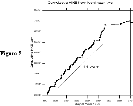
To assess whether the NIWs are important to mixing, the cumulative horizontal kinetic energy (HKE) flux from these packets was estimated (Figure 5). Each dot represents the contribution to the flux from a packet of solitons. This estimate was based on estimating the HKE in the packet assuming a propagation speed of about 0.5 m/s. The average flux is about 11 W per meter of crest-the total energy flux (including potential energy) would be at least a factor of 2 higher.
 

To determine if this flux is important to mixing, an estimate needs to be made of the distance over which these waves are dissipated. If they are gone after traveling 10 km, then the average dissipation would be 1 x 10^-3 W/m². This value is discounted if they travel farther. Most likely they do not propagate more than 50 km beyond the mooring. Is this a significant dissipation? As an internal wave enthusiast, it is tempting to compare with the internal wave energy in the deep ocean, as described by the Garrett-Munk spectrum. The value of 1 x 10^-3 W/m² is believed to be about the right order of magnitude of the energy flux through the internal wave field, dissipating the internal wave energy in 30 days. On the shelf the internal wave energy is about 10 times less, making 1 x 10^-3 W/m² dissipation relatively more important.

The importance to mixing depends upon just where and how the energy in the NIWs is lost. This is perhaps a topic for future study. Comparison with other shelf processes may provide some perspective. Hurricane Edouard passed the mooring site in September and mixed the water dramatically in about 6 hours. If the observed NIWs were to do this mixing, it would take 15 to 30 days!

A caveat on this energy flux estimate: only the "soliton" pulses were included. The lower frequency nonlinear internal tide may provide significant flux and should be counted as part of the NIW field.
 

CONCLUSIONS

Nonlinear Internal Waves are common enough to appear in observations around the world and have caught the attention of many varied disciplines. The answer to the question, Why study these waves?, will depend on the discipline responding, but two general answers are that they are interesting and important. Obviously they must be interesting, stimulating a great body of literature and generating conferences such as this one. As to importance, for physical oceanography mixing is one of the measures. They undoubtedly play an important role in specific regions at certain times, but the verdict is still out on their general importance to mixing on the shelf.